Nonlinear Electrical Impedance Tomography Method Using a Complete Electrode Model for the Characterization of Heterogeneous Domains

Jeongwoo Park,Bong-Gu Jung and Jun Won Kang

Department of Civil and Environmental Engineering,Hongik University,Seoul,04066,Korea

ABSTRACT This paper presents an electrical impedance tomography (EIT) method using a partial-differential-equationconstrained optimization approach.The forward problem in the inversion framework is described by a complete electrode model(CEM),which seeks the electric potential within the domain and at surface electrodes considering the contact impedance between them.The finite element solution of the electric potential has been validated using a commercial code.The inverse medium problem for reconstructing the unknown electrical conductivity profile is formulated as an optimization problem constrained by the CEM.The method seeks the optimal solution of the domain’s electrical conductivity to minimize a Lagrangian functional consisting of a least-squares objective functional and a regularization term.Enforcing the stationarity of the Lagrangian leads to state,adjoint,and control problems,which constitute the Karush-Kuhn-Tucker(KKT)first-order optimality conditions.Subsequently,the electrical conductivity profile of the domain is iteratively updated by solving the KKT conditions in the reduced space of the control variable.Numerical results show that the relative error of the measured and calculated electric potentials after the inversion is less than 1%,demonstrating the successful reconstruction of heterogeneous electrical conductivity profiles using the proposed EIT method.This method thus represents an application framework for nondestructive evaluation of structures and geotechnical site characterization.

KEYWORDS Electrical impedance tomography;complete electrode model;inverse medium problem;Karush-Kuhn-Tucker(KKT)optimality conditions;nondestructive evaluation of structures

1 Introduction

Electrical impedance tomography (EIT) is a nondestructive evaluation method that infers the electrical conductivity,permittivity,or impedance of structures using the surficial measurement of electrical responses due to currents.The method seeks to construct a tomographic image of an object by estimating the spatial distribution of its impedance or electrical conductivity.EIT has been recognized as a highly applicable technique in medical imaging,industrial process monitoring,and near-surface site characterization due to its ease of field experimentation,economic feasibility,and superior ability to penetrate structures.When a structure experiences electric potential difference,current flows from the point of high potential to the point of low potential.In other words,when the electric current is input to a structure,electric potential distribution is formed within the structure and on its boundary.If a structure is heterogeneous,the path of electric current is different from the homogeneous case.Therefore,the electric potential distribution of a structure depends on its material heterogeneity[1,2].

The problem of reconstructing the material properties of a structure using the measured electrical response from the surface can be defined as an inverse medium problem.Many mathematical algorithms and numerical strategies have been proposed to improve the solution to this problem.For example,mathematical and statistical regularization methods have been proposed to relieve the ill-posedness of the inverse problem and improve the solution convergence [3–6].Representative methods for solving the nonlinear EIT problem include the back-projection method [7],one-step Newton method[8],D-bar method[9],and block method[10].Recent studies have also investigated combining the EIT technique with neural networks to improve the accuracy of the tomographic image reconstruction of structures [11].Such developments have been primarily applied to medical imaging for cancer detection and brain activity imaging.In civil engineering,research on the feasibility of applying the EIT to structural condition assessment or site characterization has been increasing recently.Recent applications of the EIT to civil structures include crack detection in pipes buried in the ground [12],ground saturation monitoring,and damage detection in carbon fiber-reinforced polymer(CFRP)materials[13].To successfully implement the EIT,it is essential to have an efficient and accurate forward solver.In civil engineering applications,however,ensuring the accuracy of the forward solution remains a challenge because of the wide range of material properties,scales,and contact impedance between electrodes and structures.

For improving the previous development of the EIT for civil structures,this study proposes a nonlinear inversion method using a complete electrode model (CEM),targeting the reconstruction of the electrical conductivity profile of heterogeneous domains.The CEM comprises the Laplace equation for electric potential and the boundary conditions that express the current input to the structure via surface electrodes [14–16].Because the CEM enables the realistic modeling of the interface between the structure and electrodes,accurate solutions of the electric potential in the structural medium and the electrodes are expected.The forward solution generated by the CEM is used within the nonlinear inversion framework for reconstructing the electrical conductivity profile of structures.Specifically,the inverse problem is resolved using a partial differential equation(PDE)-constrained optimization approach.This approach seeks the optimal solution of the medium’s electrical conductivity to minimize a Lagrangian,which comprises a least-squares objective functional augmented by the weak imposition of the governing PDE and boundary conditions from the CEM.Enforcing the stationarity of the Lagrangian leads to state,adjoint,and control problems,which constitute the Karush-Kuhn-Tucker(KKT)optimality conditions.They are the first-order optimality conditions resulting from the first variation of the Lagrangian with respect to state,adjoint,and control variables.The electrical conductivity profile of the domain is then iteratively updated by solving the KKT conditions in the reduced space of the control variable.A conjugate gradient method with an inexact line search is used for the iterative solution of the electrical conductivity.To the best of the authors’knowledge,the EIT method based on the PDE-constrained optimization using the CEM and KKT conditions has been presented for the first time.The proposed inverse EIT problem deals with the Laplace equation,Robin,and Neumann boundary conditions in the PDE-constrained optimization.There are similar EIT approaches developed so far,but they mostly deal with Neumann or Dirichlet boundary conditions to solve the forward problem [17–19].Some recent studies have included the Robin boundary condition to reflect the contact impedance between the domain and electrode boundaries,but their inverse formulation and optimization schemes are different from the present study[20,21].

The remainder of this paper is organized as follows:In Section 2,the forward problem described by the CEM is presented.In Section 3,the formulation of the electrostatic inverse medium problem is presented using the Lagrangian functional and the first-order optimality conditions.In Section 4,the inversion process used to iteratively update the electrical conductivity profile in the reduced space is described.Section 5 discusses numerical examples for a series of cases in which homogeneous and heterogeneous electrical conductivity profiles are reconstructed.Finally,Section 6 presents the conclusions of the study.Finite differences for a non-unifrom grid are well shown in Figs.A1–A3.

2 Forward Problem

2.1 Problem Statement Using the Complete Electrode Model

To solve the inverse medium problem using measured electric potential values,it is first necessary to resolve the electrostatic forward problem for calculating the electric potential due to the current input.This study uses the CEM as a mathematical model for the forward problem.The CEM accounts for the current loss that occurs when the current flows to a low impedance material through an electrode and the voltage drops due to the contact impedance between the structural surface and electrode[14,22].The current loss and voltage drop influence the measured electric potential values detected by the electrodes.As the CEM considers both the contact impedance and current loss at the electrodes,the error between the calculated electric potential and the experimentally derived electric potential is generally smaller than that computed using other models.Fig.1 schematically shows a circular structure with electrodes on its surface.Solving the forward problem using the CEM reveals the electric potential inside the structure and that at the electrodes due to the current input through the electrodes.

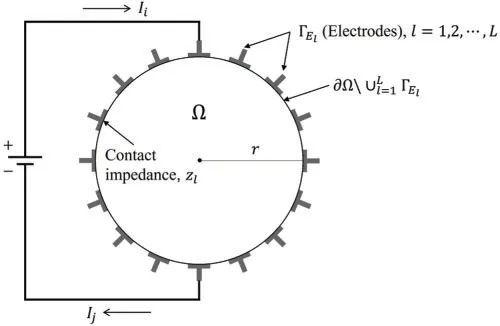
Figure 1:Schematic of a circular structure and surface electrodes

The forward problem described by the CEM can be formulated as the following boundary value problem:

where Ω denotes the structural domain,uis the scalar electric potential,σis the electrical conductivity,nis the outward unit normal on the boundary∂Ω,Eldenotes thelth electrode,ΓElis thelth electrode boundary,zlis the contact impedance ofEl,Ilis the injected current atEl,Ulis the electric potential atEl,andLis the number of electrodes.To ensure the existence and uniqueness of solutions,we add

to the model.To determine the reference point for the electric potential,

must be satisfied.We multiply Eq.(1)by a test functionv(x)and integrate it over the domain Ω,which r esults in

Using the boundary conditions(2a)and(2c),Eq.(5)can be rewritten as

Next,we integrate Eq.(2a)over ΓEl,which results in

Eq.(7)is multiplied by a test valueVl,divided byzl,and summed for all electrodes,which yields

Adding Eqs.(6)and(8)results in

Eq.(9)is the weak form of the forward problem.The electric potentialuin the domain and the potential U at the electrodes are approximated using Legendre basis functionsφi(x)and basis vectors nj,respectively:

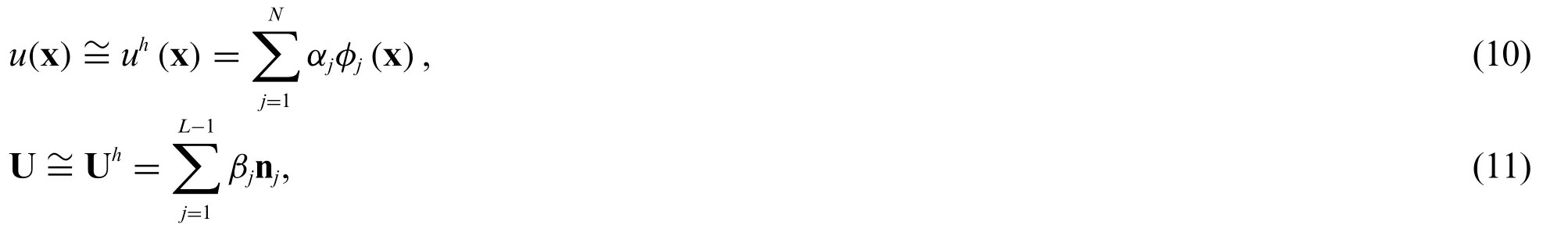
whereNis the number of nodes in the finite element mesh.The coefficientαjis the nodal value ofu(x),βjis the unknown parameter for linearly combining vectors nj,and Uhis a vector consisting of the electric potential at each electrode.The basis vectors nj∈RL×1are defined as

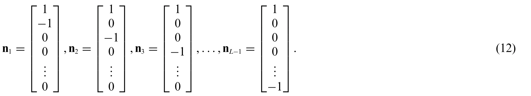
The choice of njensures that Eq.(4) is satisfied.The test functionvand the value ofVlat the electrode can be similarly approximated as

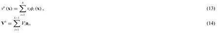
where Vhis a vector consisting of the value ofVat each electrode.By substituting Eqs.(10),(11),(13),and(14)into the weak form represented by Eq.(9),a linear system of equations for unknown vectorcan be obtained

where the matrices and vectors are written as

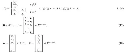
In Eq.(16d),|el|is the length of thelth electrode.Solving Eq.(15)yields nodal values of the electric

potential in the domain as well as the values ofβ.The potentialsUlhat the electrodes can be obtained as follows:

2.2 Validation of Forward Solutions

For validation,the forward solutions are compared to the solutions obtained using Technology Computer-Aided Design (TCAD) software.TCAD is used for modeling electronic design processes and the behavior of electrical devices based on fundamental physics [23].Fig.2 shows the configuration of a circular domain with a radius of 10 cm.The electrical conductivity of the domain is 1.56×10-1S/cm.A total of 16 electrodes is arranged to cover 50%of the boundary;a current of 0.78 A is input into the fifth electrode,and it flows out through the 13th electrode.The contact impedance of the electrodes is 9.8×10-7Ω·cm2.In this case,the potential of the fifth electrode is 10 V.Fig.3 shows the distribution of the calculated electric potential within the domain due to the current input.The numerical solution calculated using the CEM is very close to the result obtained using the TCAD software.

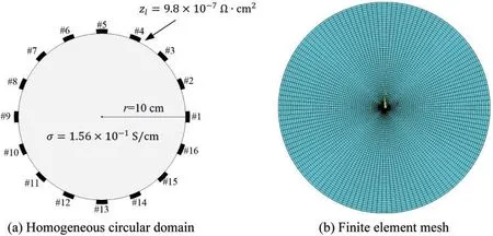
Figure 2:Homogeneous circular domain and finite element mesh for validating the forward solution

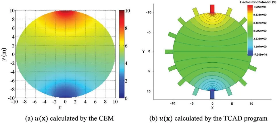
Figure 3:Calculated electric potential,u(x),in the homogeneous circular domain

The error of the forward solution relative to the TCAD result can be calculated using the following equation:

Table 1 shows the electric potential values at each electrode and the corresponding relative errors.The maximum error is 3.37%,which demonstrates the accuracy of the forward solution.Fig.4 depicts the electric potential,Ul,calculated at each electrode.

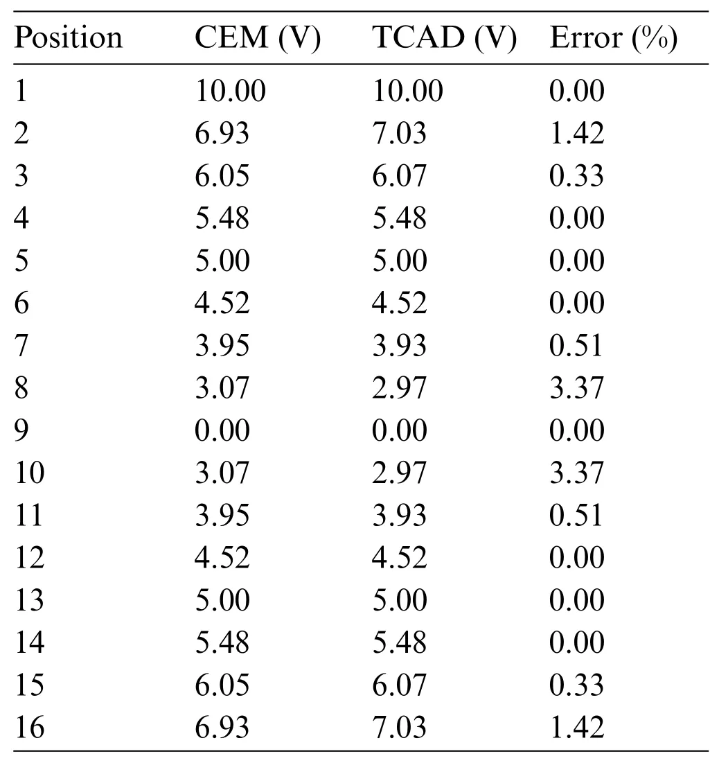
Table 1:Electric potential values at each electrode (calculated using the CEM and TCAD) and the corresponding relative errors

Figure 4:Graphical representation of the electrical potential at each electrode

2.3 Mesh-Type Dependency of the Forward Solution

For investigating the dependency of the forward solutions on the finite element mesh,two mesh types are explored:a radial mesh composed of eight-node quadrilateral elements and a mixed mesh with a square section inside.Fig.5 illustrates these two types of meshes.

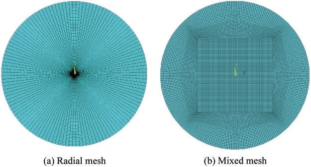
Figure 5:Two finite element mesh types for forward and inverse analyses

Fig.6 shows a circular domain with a radius of 15 cm and electrodes attached to its boundary.The domain is assumed to be homogeneous,with an electrical conductivity of 1×10-2S/cm,which is typical of concrete materials.A total of 32 electrodes is arranged on the boundary and are spaced evenly to cover 50% of the boundary (as for the domain described in Section 2.2).A current with a cosine pattern along the perimeter is input to each electrode.The magnitude of the current at each electrode isIl=cos(2πl/L),whereLis the total number of electrodes,andlis the index for the electrode number.The contact impedance of the electrodes is 0.22 Ω·cm2.Fig.7 presents the forward solutions calculated using the two meshes displayed in Fig.5.Fig.7c shows the calculated electric potential values at the electrodes on the boundary.The two results show that the forward solution changes minimally with the mesh type.

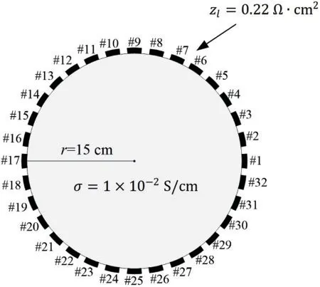
Figure 6:Homogeneous circular domain with 32 electrodes on the boundary

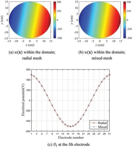
Figure 7:Forward solutions calculated using the two meshes

3 Inverse Problem

3.1 PDE-Constrained Optimization

The problem of reconstructing the electrical conductivity profile of a structure using the electric potential measured at surface electrodes can be formulated as the following PDE-constrained optimization problem:

The objective functionalJconsists of a misfit functional in a least-squares sense and a regularization termγ(σ).The misfit functional is expressed as the sum of the squared differences between the calculated electric potentialUland the measured electric potentialUmlat electrodeEl.This optimization problem is constrained by the governing Eq.(1)and boundary conditions(2)–(4)of the forward problem.To relieve the ill-posedness of the inverse problem,the regularization termγ(σ)is included in the objective functionalJ.In this study,the Tikhonov(TN)regularization scheme is used;thus,the regularization term can be written as

whereRσis a regularization factor that controls the penalty to the gradient of the electrical conductivityσ(x).Although TN regularization cannot accurately capture sharply varying material profiles,it still assists the inversion process in narrowing the feasibility space of solutions and improving the solution convergence.

3.2 First-Order Optimality Conditions

The PDE-constrained optimization problem can be converted to an unconstrained optimization problem using a Lagrange multiplier method.Specifically,the objective functionalJcan be augmented by Eqs.(1)and(2b)to construct the Lagrangian functionalL,

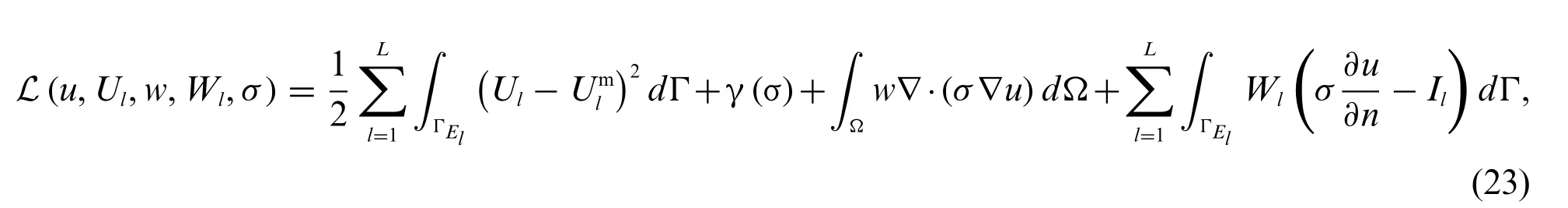
wherewandWlare Lagrange multipliers applied to the left-hand terms of the governing equation and boundary conditions,respectively.The electrical conductivityσ(x)that minimizes the Lagrangian is the solution to the inverse problem.For the optimal solutions,first-order optimality conditions are introduced,which enforce the first variation of the Lagrangian with respect to state variablesuandUl,adjoint variableswandWl,and the control variableσto vanish.

3.2.1 First Optimality Condition:State Problem

At the optimum of the Lagrangian,its first variation with respect to the adjoint variableswandWlshould vanish.Introducing the stationarity conditionsδwL=0,δWlL=0,andl=1,2,...Lresults in the state problem,which is identical to the forward problem presented in Eqs.(1)and(2).

3.2.2 Second Optimality Condition:Adjoint Problem

At the optimum of the Lagrangian,its first variation with respect to the state variablesuandUlshould vanish as well.Applying the stationarity requirements,δuL=0,δUlL=0,andl=1,2,...L,to the Lagrangian yields

BecauseδuandδUl (l=1,2,...L)are arbitrary,Eq.(24)results in the following adjoint problem:

Eq.(25) is the governing equation for adjoint variablew(x),and Eqs.(26a)–(26c) are boundary conditions forw(x)andWl.Eq.(26b)indicates the source of the adjoint problem,which depends on the potential misfit at the electrodes.The adjoint problem has the same differential operators as the state problem does.

3.2.3 Third Optimality Condition:Control Problem

Finally,the first variation of the Lagrangian with respect to the control variableσshould vanish at the optimum.Introducing the stationarity condition(δσL=0)to the Lagrangian results in

Becauseδσis arbitary,Eq.(27)yields the following control problem:

The control problem is a boundary value problem for the electrical conductivityσ(x),with Eq.(28)being the governing equation and Eqs.(29a)and(29b)being the boundary conditions.The solutionσ(x)can be calculated once the state and adjoint solutionsu,w,andWlare obtained.The state,adjoint,and control problems constitute the KKT conditions for the PDE-constrained optimization problem.

4 Inversion Setup and the Simulation Process

4.1 Finite Element Formulation of the Adjoint Problem

The adjoint problem described in Section 3.2.2 can be solved using the Galerkin finite element method.Specifically,Eq.(25)is multiplied by a test functionv(x)and integrated over the entire domain Ω.Upon integrating the resulting equation by parts and using a procedure similar to that represented by Eqs.(5)to(9),the weak form of the adjoint problem can be derived as

whereVlis a test value used to derive the weak form of Eq.(26a).The adjoint solutionswandWlcan be approximated using Legendre basis functionsφi(x)and basis vectors nj,respectively,as follows:

whereis the nodal value ofw(x),is the unknown parameter for linearly combining vectors nj,and Whis a vector consisting ofWlat each electrode.The test functionsvandVlare approximated using Eqs.(13)and(14).

Substituting Eqs.(13),(14),(31) and (32) into (30) results in the following linear system of equations:

where Kadj,uadj,and Fadjare the stiffness matrix,solution vector,and right-hand side vector of the adjoint problem,respectively.The superscript “adj”denotes the adjoint problem.The matrices and vectors in Eq.(33)can be written as

Solving Eq.(33)yields nodal values of adjoint variablewin the domain as well as the values ofβadj.The adjoint variableWlhat the electrodes can be derived as

The submatrices in Eq.(33)are related to those of the state problem through

Eq.(38)contributes to reducing the computational cost of constructing the system matrices of the adjoint problem in the inversion process.

4.2 Material Property Update

By solving the state and adjoint problems,the first and second optimality conditions are satisfied.Only the true profile ofσ(x)exactly satisfies the control problem represented by Eqs.(28) and(29).Therefore,the material profileσ(x)must be updated to satisfy the third optimality condition.Updatingσ(x)to minimize the LagrangianLrequires a reduced gradient forL.The process of updating the control variableσ(x)using the state and adjoint solutions can be summarized as follows:

1)Assuming the initial profile ofσ(x),solve the forward problem(1)and(2)for state variablesu(x)andUl.

2)Using the state solutionUl,solve the adjoint problem(25)and(26)for adjoint solutionsw(x)andWl.

3)Using the state and adjoint solutions,calculate the reduced gradient forLwith respect to the control variableσ(x)as

where the derivatives are calculated using second-order accurate finite difference methods.When using a radial mesh,such as that shown in Fig.5a,the reduced gradient (40) expressed in a cylindrical coordinate system can be used

4)Determine the search direction using a line search method and update the electrical conductivity profileσ(x).

4.2.1 Conjugate Gradient Method with Inexact Line Search

In this study,the search direction for the optimal solution of the control variableσis determined using the Flétcher-Reeves conjugate gradient method with an inexact line search.The continuous form of the reduced gradient,Eqs.(39)or(40),can be discretized by being evaluated at each nodal point.Let gkdenote the discrete reduced gradient at thekth inversion iteration,

Then,the electrical conductivity vectorσkcomprising nodal values ofσis updated via

where dkis a search direction vector atσk,andαis the step length in the direction of dk.By using the Flétcher-Reeves method,the search direction vector is calculated as

The misfit functional is evaluated using the updated electrical conductivityσk+1and is compared to a preset tolerance.If it does not meet the tolerance criterion,the inversion process setk←k+1 and proceeded to the next iteration.As is known,the discrete search direction vector dkgradually deviates from the direction to a local minimum because of the non-optimal step lengthαand the round-off error arising from the accumulation of the gk·gk/gk-1·gk-1terms in Eq.(43).Therefore,it is necessary to reset dm+1to-gm+1after everymth iteration.

In this study,an inexact line search method is used to determine a step lengthαthat would yield an adequate reduction in the objective functionalJ.Specifically,the method requires the step length to reduce the objective functional sufficiently,as indicated by theArmijo condition(orsufficient decrease condition);this condition is expressed as

whereis selected to be a small value,which is=10-10in this study.To satisfy the Armijo condition,the backtracking algorithm described in Table 2 can be used.In this procedure,an initial step lengthis set at the beginning.If Eq.(44)is violated during the inversion,the step length is iteratively reduced by settingα←.In this study,=0.5 is used.

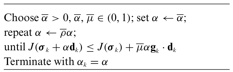
Table 2:Backtracking algorithm to determine the step length α

4.2.2 Regularization Factor Continuation Scheme

The choice of the regularization factorRσin Eqs.(39)or(40)considerably affects the reconstruction of the electrical conductivity profile.IfRσis excessively large,it may be difficult to capture a sharply varying interface in the profile because of the large penalty on the gradient ofσ(x).Conversely,ifRσis excessively small,the inversion may suffer from a solution multiplicity problem.To determine the optimal regularization factor at each inversion iteration,a regularization factor continuation scheme [24–26] is used in this study.The reduced gradient in Eqs.(39) or (40) can be formally rewritten as

in which

In Eq.(45),Rσ(∇σJr)represents the gradient of the regularization functional,and ∇σJmdenotes the gradient of the misfit functional.The first term,Rσ(∇σJr),penalizes spatial oscillations in the inverted profile such that an increasingRσresults in a smoother inverted profile.A balance between these two terms can be imposed using

Therefore,Rσcan be calculated at each iteration as

where the value of the weight factorεis between 0.5 and 1,as recommended for a reasonable regularization effect.

5 Numerical Results

5.1 Homogeneous Domains

Consider a circular domain with a radius of 15 cm,as shown in Fig.8.A total of 32 electrodes is placed on the boundary and spaced evenly to cover 50% of the boundary.For finite element implementation,the mixed mesh illustrated in Fig.5b is used.The contact impedance of the electrodes is 0.22 Ω·cm2.The initial value of the regularization factorRσis 1.0,and the weight factorεfor the regularization factor continuation scheme is 0.5.As an excitation to the domain,a current with a cosine pattern,as expressed in Eq.(49),is input to each electrode along the circular perimeter,

Fig.9 shows the target,initial guess,and reconstructed electrical conductivity profiles.The target profile is homogeneous withσtg=1.0 S/cm,which is typical of graphite materials.The inversion starts with an initial guess ofσini=0.5 S/cm and reconstructs the target profile accurately at about 700 iterations.Fig.9d shows the response misfit as a function of the iteration number during the inversion process.The misfit decreases from 3×102to 1.49×10-3,which represents a reduction on the order of 10-5.The response misfit,Fm,as part of the objective functionalJin Eq.(21),can be written as

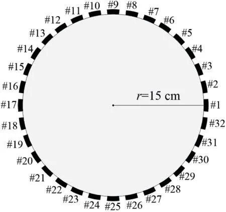
Figure 8:Schematic of a circular domain and 32 surface electrodes used for inversion

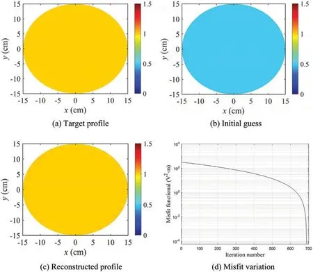
Figure 9:Numerical inversion for homogeneous target profile

To investigate the accuracy of the inversion result,the errors in the inverted electrical conductivity values are calculated at four sampling points,as shown in Fig.10:A(0,0),B(4,0),C(8,0),and D(12,0).Table 3 lists the errors at each sampling point.The maximum error is 0.116%,which demonstrates that the inversion for the homogeneous electrical conductivity profile is highly accurate.

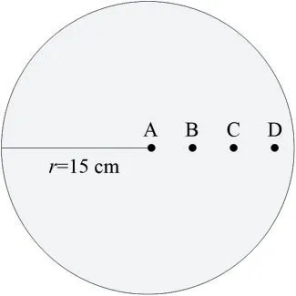
Figure 10:Sampling points for error calculation

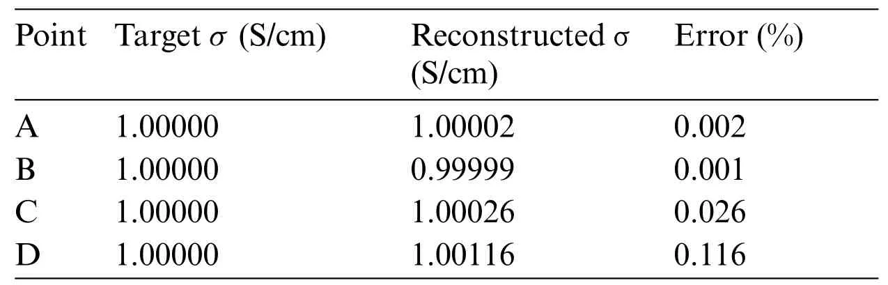
Table 3:Errors in the inverted electrical conductivity values at the sampling points(inversion case with σtg=1.0 S/cm and σini=0.5 S/cm)

To investigate the effect of the initial guess on the reconstructed profile,four cases of the inversion with different initial-to-target ratios are considered.Table 4 shows the four cases for the initial guessσiniand targetσtg.For Cases 1 and 2,the initial guess is less than the target,whereas for Cases 3 and 4,it is greater.The electrode arrangement,input current,and contact impedance are the same as those in the previous example.

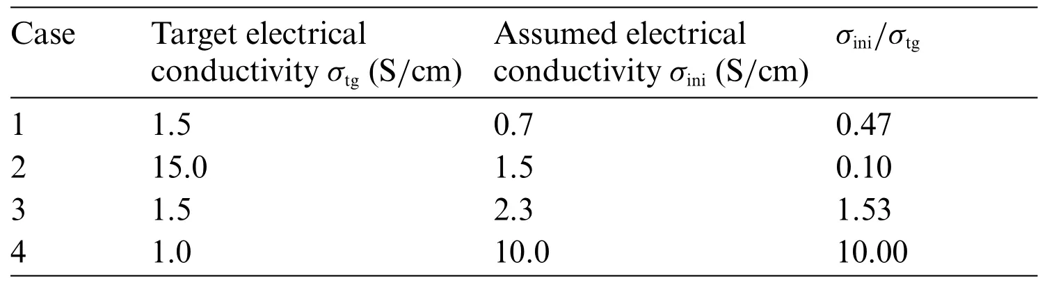
Table 4:Four cases of inversion with different initial-to-target ratios

Figs.11–14 display the inversion results for the four electrical conductivity profiles presented in Table 4.In all four cases,the homogeneous target values are accurately reconstructed.In particular,as shown in Figs.12b and 14b,the target values are recovered well even when the target is 10 times smaller or larger than the initial guess.Figs.11c,12c,13c and 14c show the misfitFmas a function of the number of iterations.For each case,the misfit decreases by a factor of at least 10-5.Figs.11d,12d,13d and 14d show the electric potential values at the 32 electrodes calculated using the reconstructed electrical conductivity profile for each case.The calculated electric potential values nearly coincide with the measured values,which demonstrates that the target profiles are successfully reconstructed.The root-mean-square(RMS)error,eRMS,and the relative RMS error,er,RMS,of the electric potential at the electrodes can be calculated using Eq.(51).In the equations,UiandUimdenote the calculated and measured electric potential values at theith electrode,respectively,and |is the absolute maximum of the measured potentials.Table 5 shows the calculated RMS errors for each case of the inversion process.Even in Case 4 with the largest relative error,the value is less than 0.18%.In all cases,the inversion results are evaluated to be sufficiently accurate,

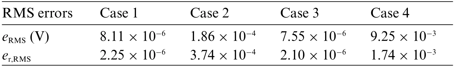
Table 5:RMS errors of the reconstructed homogeneous profiles

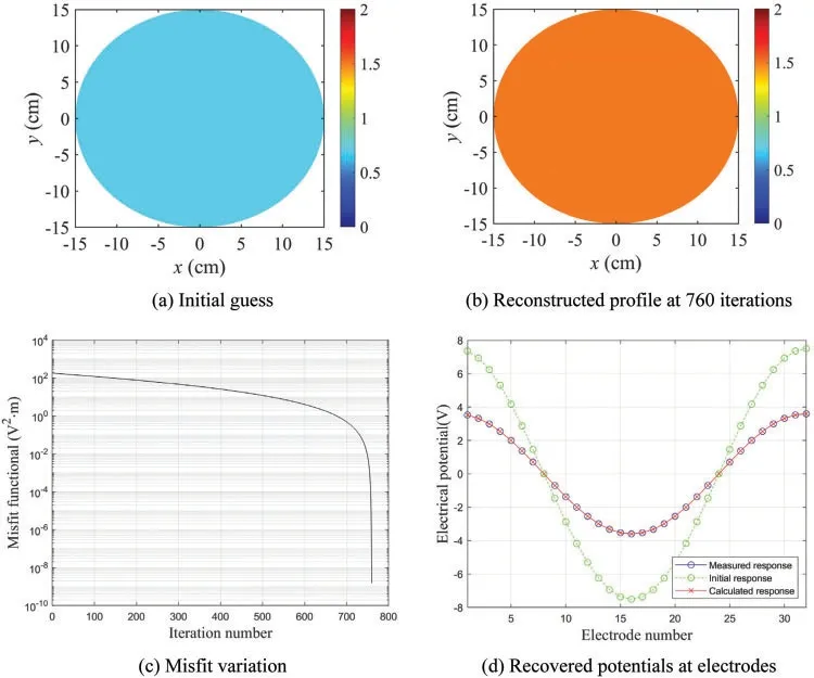
Figure 11:Inversion results for Case 1;σtg=1.5 S/cm,σini=0.7 S/cm

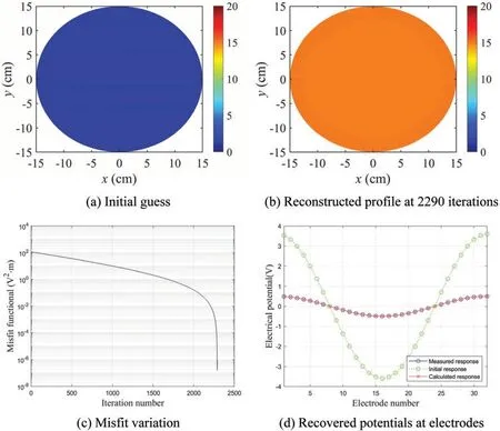
Figure 12:Inversion results for Case 2;σtg=15.0 S/cm,σini=1.5 S/cm

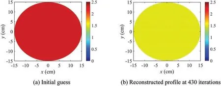
Figure 13:(Continued)

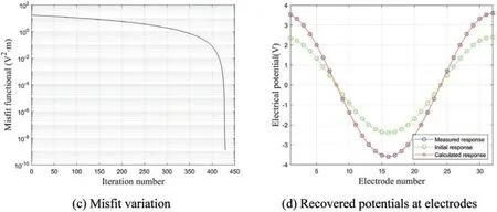
Figure 13:Inversion results for Case 3;σtg=1.5 S/cm,σini=2.3 S/cm

Figure 14:Inversion results for Case 4;σtg=1.0 S/cm,σini=10.0 S/cm

5.2 Heterogeneous Domains

Next,the inversion is performed to reconstruct heterogeneous electrical conductivity profiles.Fig.15 shows three cases of the target profile.In Case 5,the target values of the electrical conductivity are 0.04 S/cm fory≥0 and 0.01 S/cm fory ＜0.In Case 6,the target profile is divided into three layers:0.04 S/cm fory≥5,0.025 S/cm for-5 ≤y ＜5,and 0.01 S/cm fory ＜-5.The target profile for Case 7 has four quadrants.In quadrants 1 and 3,the target value is 0.04 S/cm.In quadrants 2 and 4,the target value is 0.01 S/cm.The target conductivity values of Case 5 to Case 7 are typical of air-dried concrete materials in various conditions [27].Examples of the profile heterogeneity in Fig.15 include fiber-reinforced composite sandwich plates and concrete specimens under curing.The electrode arrangement,current input,contact impedance,initial value ofRσ,and weight factorεare the same as in the homogeneous domain cases.

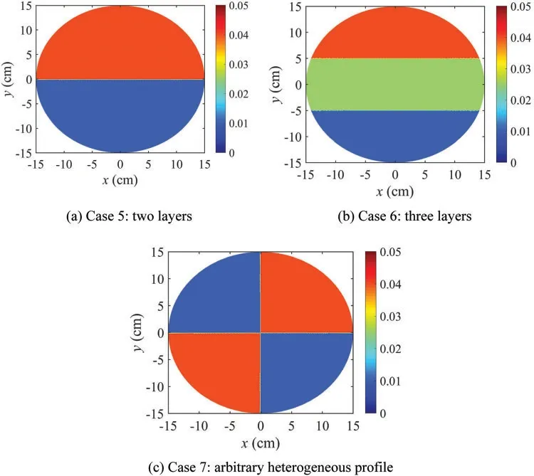
Figure 15:Heterogeneous target electrical conductivity profiles

Figs.16–18 show the inversion results for the heterogeneous electrical conductivity profiles.The target conductivity values are reconstructed reasonably well in the three heterogeneous cases.Figs.16c,17c,and 18c show the response misfitFmas a function of the iteration number.Figs.16d,17d,and 18d show the electric potential values calculated at the electrodes using the reconstructed electrical conductivity profile for each case.The calculated electric potential values nearly coincide with the measured ones,which demonstrates that the reconstructed profiles converged to the targets.For each case,the initial misfit decreases by a factor on the order of 10-3.Table 6 shows the RMS error and the relative RMS error of the electrical potentials calculated at the electrodes for each case.The errors were calculated using Eq.(51).They are relatively large compared with those in the homogeneous cases,due to the difficulty in accurately recovering the sharply varying interfaces between layers.Nevertheless,the relative RMS error of the heterogeneous cases is less than 0.80%,indicating that the inversion results are sufficiently accurate.

Table 6:RMS errors of the reconstructed heterogeneous profiles

Figure 16:Inversion results for Case 5

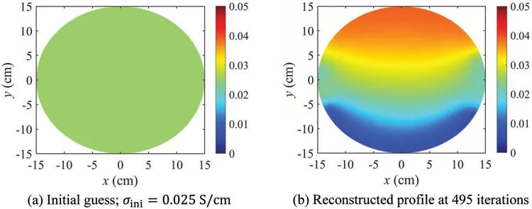
Figure 17:(Continued)

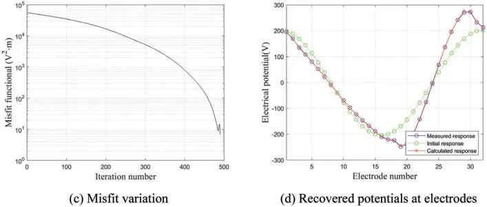
Figure 17:Inversion results for Case 6

Figure 18:Inversion results for Case 7

6 Conclusions

This study was conducted to develop a nonlinear inversion method for electrical impedance tomography of structures using measured electric potentials at the surface.The proposed method minimizes the misfit between calculated and measured electric potential values at surface electrodes within a PDE-constrained optimization framework.The CEM was used as a forward model to calculate the electric potential due to current input.By solving the KKT conditions of the Lagrangian iteratively,the inversion procedure could successfully recover heterogeneous electrical conductivity profiles.The TN regularization scheme was used to mitigate the ill-posedness of the inverse problem and improve the convergence of the solution.A series of numerical results showed that the homogeneous and heterogeneous electrical conductivity profiles were successfully reconstructed using the inversion method developed in this study.

For all numerical example cases,the misfit was decreased from its original value by a factor on the order of 10-4or less.In addition,the electric potential values at the electrodes that were calculated using the reconstructed conductivity profiles were nearly identical to the measured values.Specifically,the relative RMS error of the calculated electric potential after inversion was less than 0.18%for the homogeneous cases.The relative RMS error of the heterogeneous cases was less than 0.80%,indicating that the inversion results are sufficiently accurate.This study is expected to provide an application framework for nondestructive evaluation of structures,geotechnical site characterization,etc.

Funding Statement: This research was funded by the National Research Foundation of Korea,the Grant from a Basic Science and Engineering Research Project (NRF-2017R1C1B200497515),and the Grant from Basic Laboratory Support Project(NRF-2020R1A4A101882611).The supports are greatly appreciated.

Conflicts of Interest:The authors declare that they have no conflicts of interest to report regarding the present study.

Appendix A.Finite Differences for a Non-Unifrom Grid

In a uniform finite-element mesh,as shown in Fig.A1,the first-order and second-order derivatives at node(i,j)can be calculated using the central difference method,as shown in Eqs.(A1)–(A4):

where Δxand Δyare the spacing between node(i,j)and the adjacent nodes in thexandydirections,respectively.For nodes located at the boundary,derivatives cannot be calculated using the central difference method,as adjacent nodes exist in only one direction.

Figure A1:Uniform finite element mesh

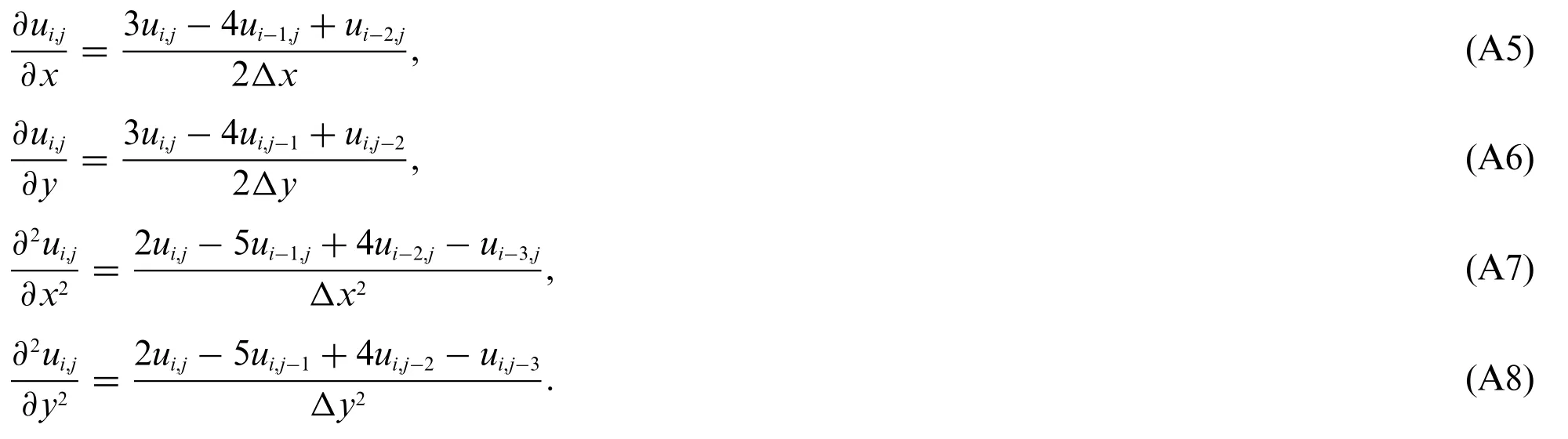
This study used the backward difference method shown in Eqs.(A5)–(A8) to calculate the derivative at nodes located at the boundary:

For a radial finite-element mesh such as that shown in Fig.A2,the polar coordinate system can be used to calculate the derivative.

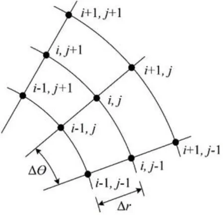
Figure A2:Polar coordinate system finite element mesh

The central difference method for the polar coordinate system is shown in

whererandθare the radial and angular coordinates,respectively.The backward difference method for the polar coordinate system can be expressed as

In a non-uniform finite-element mesh,as shown in Fig.A3,the spacing of the adjacent nodes on the left and right or above and below may differ.For such a finite element mesh,the finite difference method was used to calculate the derivatives,as shown in

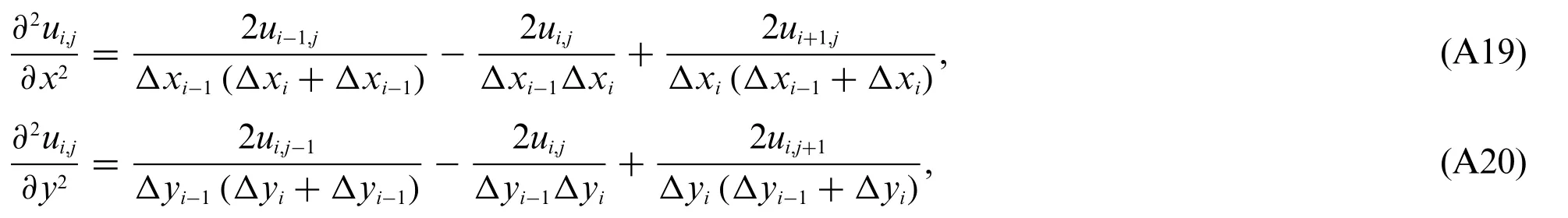
where Δxi-1is the spacing between nodes(i-1,j)and(i,j),and Δxiis the spacing between nodes(i,j)and (i+1,j);Δyi-1is the spacing between nodes (i,j-1) and (i,j),and Δyiis the spacing between nodes(i,j)and(i,j+1).

Figure A3:Non-uniform finite element mesh