A Study of Traveling Wave Structures and Numerical Investigation of Two-Dimensional Riemann Problems with Their Stability and Accuracy

Abdulghani Ragaa Alharbi

Department of Mathematics,College of Science,Taibah University,Al-Madinah Al-Munawarah,42353,Saudi Arabia

ABSTRACT The Riemann wave system has a fundamental role in describing waves in various nonlinear natural phenomena,for instance,tsunamis in the oceans.This paper focuses on executing the generalized exponential rational function approach and some numerical methods to obtain a distinct range of traveling wave structures and numerical results of the two-dimensional Riemann problems.The stability of obtained traveling wave solutions is analyzed by satisfying the constraint conditions of the Hamiltonian system.Numerical simulations are investigated via the finite difference method to verify the accuracy of the obtained results.To extract the approximation solutions to the underlying problem,some ODE solvers in FORTRAN software are applied,and outcomes are shown graphically.The stability and accuracy of the numerical schemes using Fourier’s stability method and error analysis,respectively,to increase the reassurance are investigated.A comparison between the analytical and numerical results is obtained and graphically provided.The proposed methods are effective and practical to be applied for solving more partial differential equations(PDEs).

KEYWORDS The Riemann wave equation;Hamiltonian system;solitary solutions;numerical solutions;stability;accuracy

1 Introduction

Diverse phenomena in nature and technology are described using nonlinear evolution equations(NLEEs).In physics,for instance,the heat transfer and the traveling wave phenomena are successfully modeled by PDEs.In chemistry,the dispersion of a chemically reactive substance is controlled by PDEs.Also,PDEs are invoked to characterize population growth problems.Moreover,most physical incidents of shallow-water waves,quantum mechanics,plasma physics,electricity,fluid dynamics,and more others are investigated using PDEs.In order to better comprehend the qualitative characteristics of such equations,one can study their analytical solutions.A distinct range of traveling wave structures allows us to explain the mechanisms of immense complicated phenomena.As a result,some researchers have revealed numerous effective methods.Some of the powerful approaches are the Sine-Gordon expansion approach [1],the modified simple equation technique [2],the tanh-sech process[3,4],the trial equation method [5],theexp(-f(ζ))-expansion principal [6,7] and the generalized exponential rational function approach[8].More methods can be easily seen in references[9–15].

The Riemann wave system[16,17]is given by

whereα,βandγare constants.System (1) describes a(2 + 1)-dimensional interaction for the propagation of Riemann waves in thex-axis andy-axis.The Riemann wave equations have been investigated by some scientists using various methods.For example,Shao[18]examined the stability of the solution of the quasi-linear hyperbolic systems under the influence of some BV perturbations.Shao [19] presented several solutions with satisfying some conditions.Chen et al.[20] used the generalized expansion approach of the Riccati equation to extract some soliton-like solutions for Eq.(1) whenm=n=4b,wherebis a constant.The modified mapping principle was applied in[21]to establish a class of periodic wave solutions in terms of the Jacobi elliptic functions.Moreover,Abdelrahman et al.[22] utilized the singular manifold technique to construct two general solutions for system (1).Every obtained solution contains two arbitrary functions.Then,some periodic wave solutions were derived from the obtained general solutions.In[16],the tanh method was implemented to generate some traveling wave solutions for Eq.(1).The generalized Kudryashov approach was applied in[17]to systematically and graphically show the traveling wave solutions of Eq.(1).While,in this paper,we present analytical and numerical solutions to Eq.(1)using the generalized exponential rational function approach[8]and finite difference methods,respectively.

Since our knowledge of constructing exact solutions for the Riemann wave equations is basically based on few techniques,we utilize the generalized exponential rational function approach [8]to construct the exact solutions of the considered equations.This technique depends on Jacobi elliptic functions.As a result,various solitary traveling wave solutions can be simply generated in terms of trigonometric and hyperbolic functions.Regarding the numerical solution,some numerical simulations are presented using the finite difference method to emphasize that the obtained results are accurate.The numerical solutions of the considered system are obtained by approaching the equations on a mesh using the finite-difference notations.The domain is divided into a limited set of grids to achieve meshes for both independent variablesxandy.It is well known that the wave of the solutions has areas with rapid spatial changes,for instance,steep fronts structures.In order to resolve these types of areas,fine numbers of grids,forxandy,are required.The step size,Δx=xi-xi-1,Δy=yi-yi-1should be extremely small to catch these regions.Computationally,it is intensive and expensive.Hence,I strive to achieve an alternative discretizing for the meshes to have a non-uniform mesh that manually sets more grids in where the solution varies rapidly and fewer grids outside these regions.And then,I used the stiff ODE solver DASPK[23]to solve the obtained ODEs of the semi-discretization of the system.This ODEs solver is an implicit iterative method,based on the Krylov subspace method.They are applied to solve the system of linearized equations.They also allow converting the Jacobian matrix to be LU factorized to make the calculations faster.I additionally studied,here,the stability and the error analysis for the numerical schemes.

2 Methodology

The generalized exponential rational function approach is comprehensively summarized in this section,as presented in[8].Assume that is a given nonlinear PDE in the unknown functionsV=V(x,y,t),U=U(x,y,t)andΓ=Γ(x,y,t).Pis a polynomial inV,UandΓand their partial derivatives.Suppose thatζ=μx+δy-wt,whereμ,δandware unknown parameters that will be computed later.Thus,

Then,Eq.(2)is converted into

where′=According to the proposed method,the formal solution of Eq.(4)is written as

wherep1p2,p5,p6,q1,q2,q3,andq4are complex(or real)constants so that Eq.(2)is expressed as

The balance principle is used to determine the value ofNappearing in Eq.(6).Moreover,the coefficientsA0,AkandBk(k=1,2,...,N)is evaluated such that Eq.(6) satisfies Eq.(4).Inserting Eq.(6) into Eq.(4) gives a polynomial from which one can obtain an algebraic system solved using Mathematica or Maple.The values of the above-mentioned constants are included in the solutions of this system.Substituting these values into Eq.(6)yields the exact solutions of Eq.(2).

3 Traveling Wave Solution

In this section,we study the exact solutions of system(1)using the generalized exponential rational function approach.Substitute Eq.(3)into system(1)to have

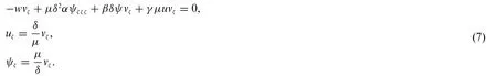
We now integrate each equation in system(7)with respect toζto obtain

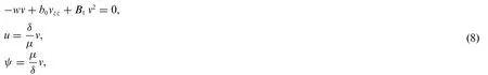
whereb0=αμ2δandB1=0.5δ(β+γ).Balancing the highest order ofvζζwith the nonlinear termv2in system(8)evaluates the value ofNgiven byN=2.As a result,the exact solutions are shown as follows:

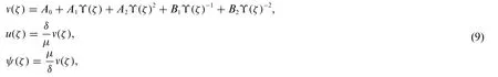
whereϒ(ζ)is presented in Eq.(5).We insert systems(9)into(8)to obtain the traveling wave solutions of(1)which are written as follows.

Family 1:Forp=[1,-1,1,1]andq=[-1,1,-1,1],Eq.(5)becomes

Substituting Eq.(10) into the first equation of system (9) and then we insert the result into the first equation of system(8)give an algebraic system whose solutions are given as follows:

Case 1:

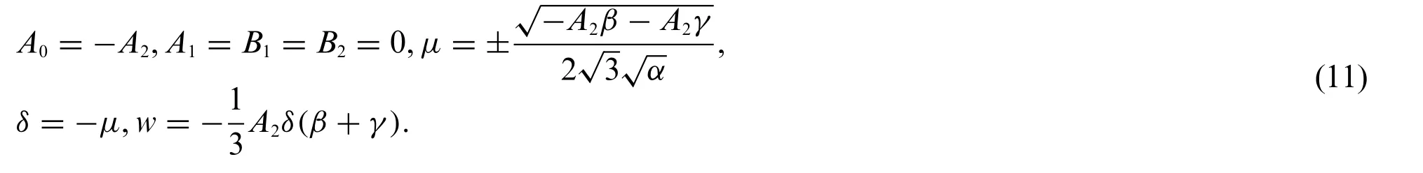
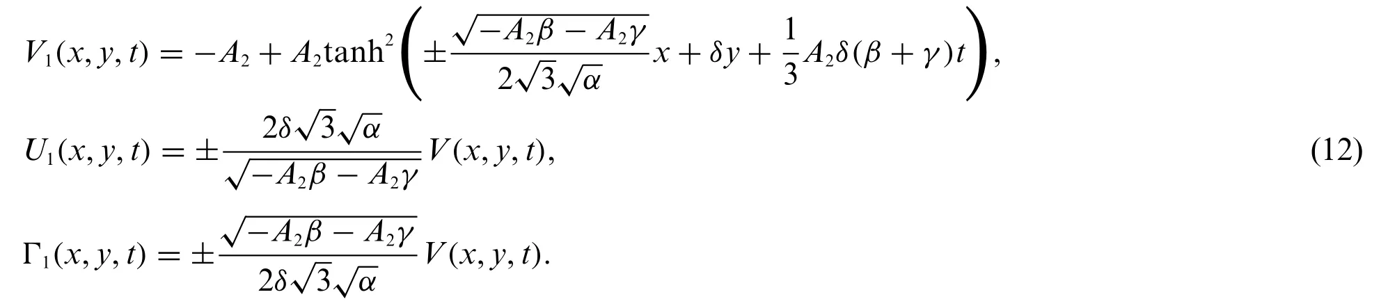
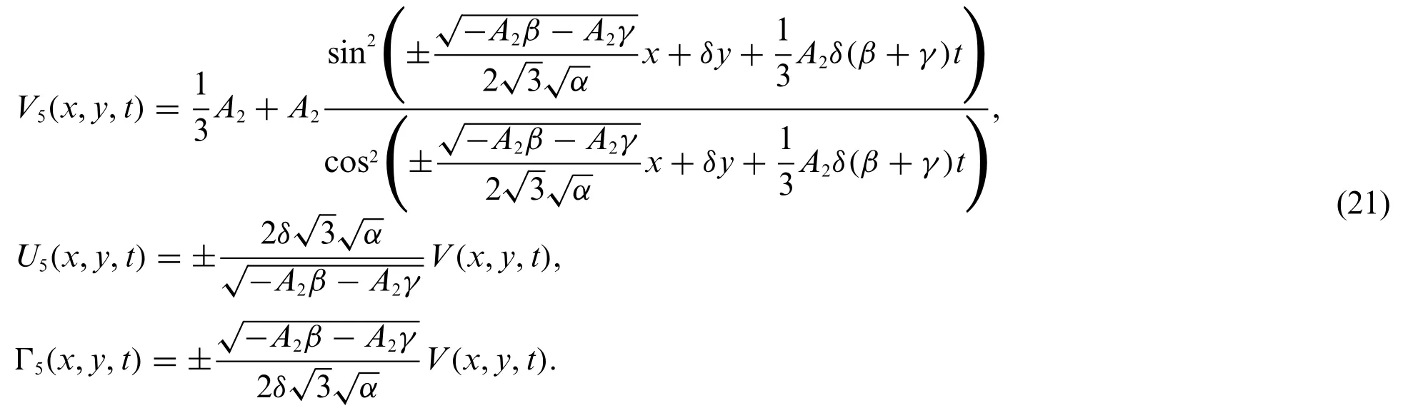
Substituting Eq.(11)into system(9)and Eq.(10)gives the exact solutions of system(1)which are illustrated as follows:

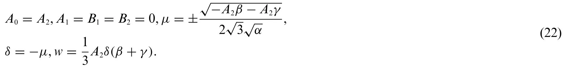
Case 2:

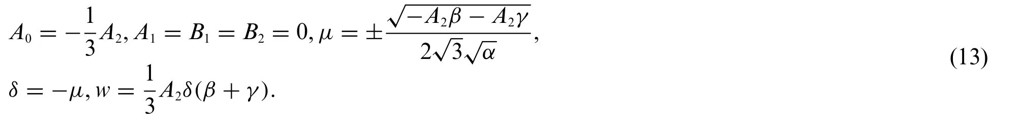
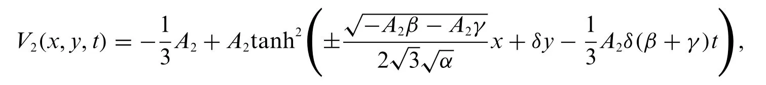
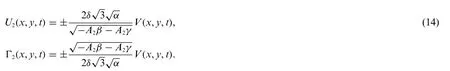
Inserting Eq.(13)into system(9)and Eq.(10)yields the exact solutions of system(1)which are expressed as

Case 3:

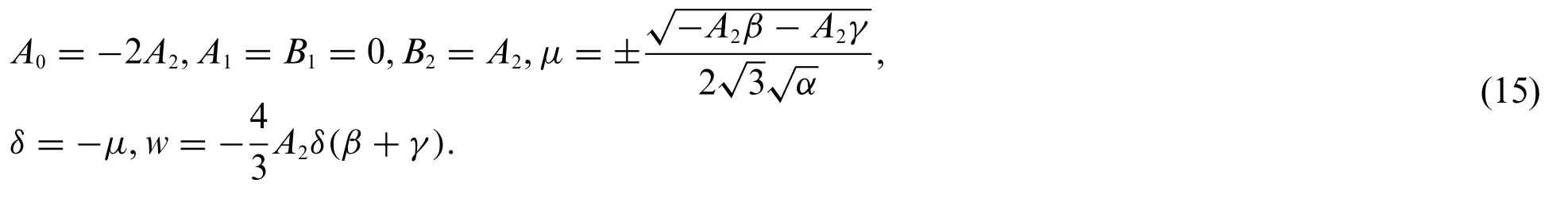
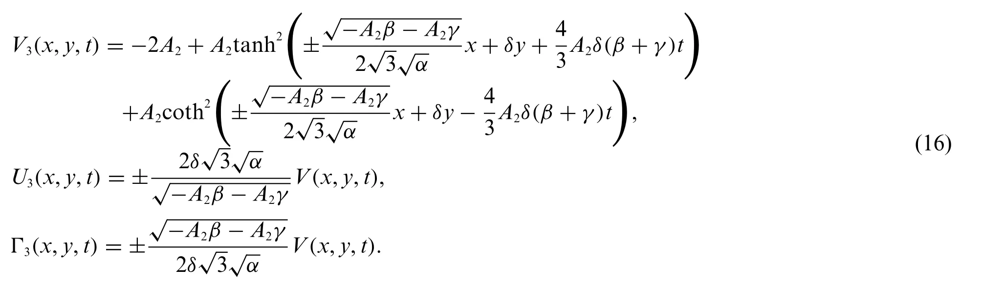
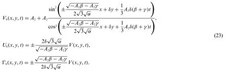
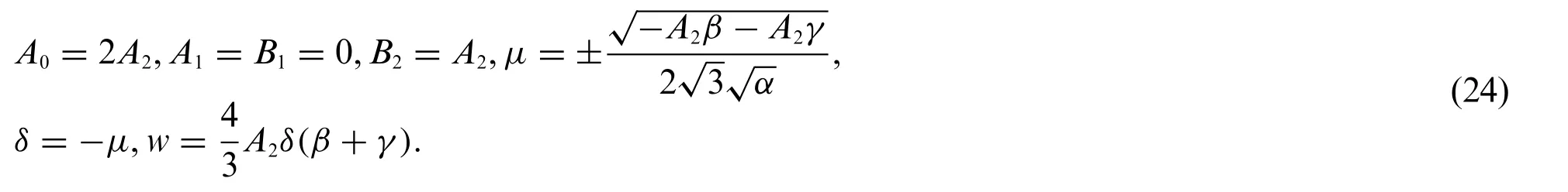
Plugging Eq.(15) into system (9) and Eq.(10) gives the traveling wave solutions of system (1)which are given by

Case 4:

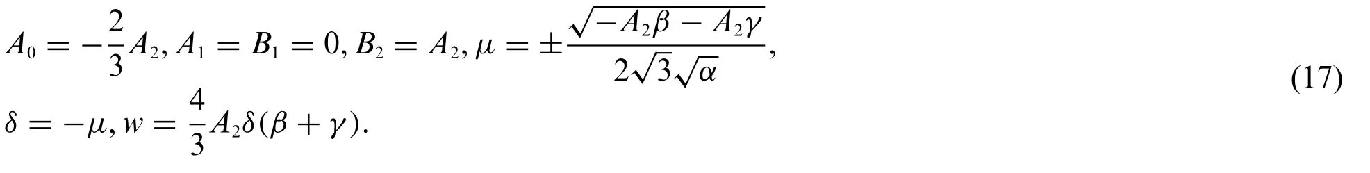
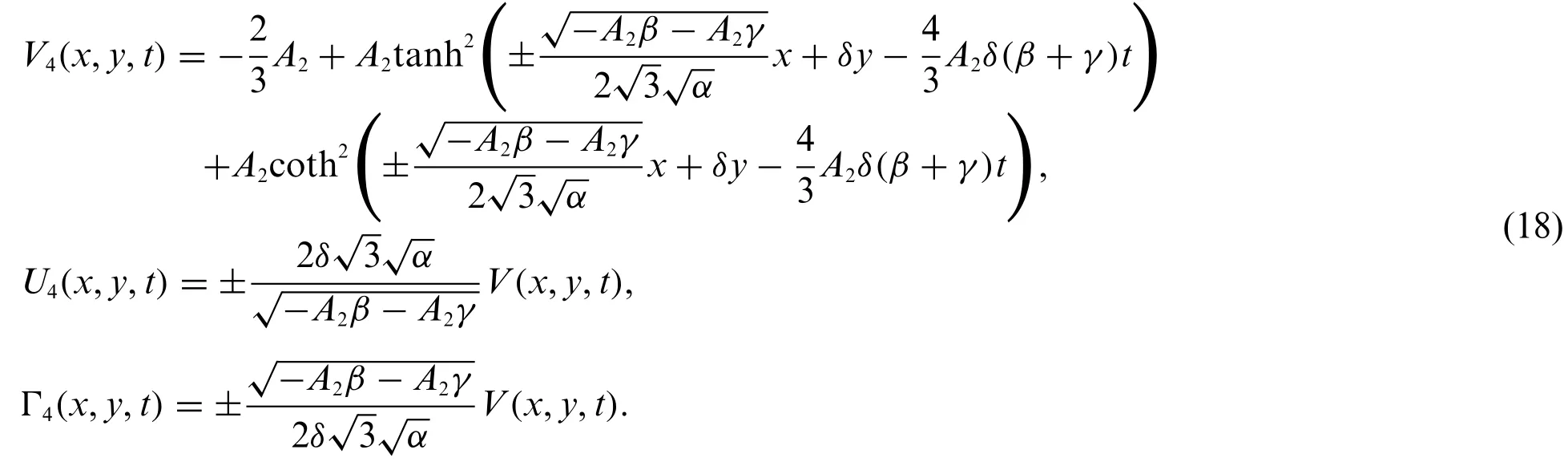
Putting Eq.(11)into system(9)and Eq.(10)leads to the exact solutions of system(1)which are shown as

Family 2:Forp=[i,-i,1,1]andq=[i,-i,i,-i],Eq.(5)becomes

Case 1:

Substituting Eq.(20)into system(9)and Eq.(19)gives the exact solutions of system(1)which are shows as follows:

Case 2:

Inserting Eq.(22) into system (9) and Eq.(19) yields the traveling wave solutions of system (1)which are

Case 3:

Putting Eq.(24)into system(9)and Eq.(19)gives the exact solutions of system(1)which are

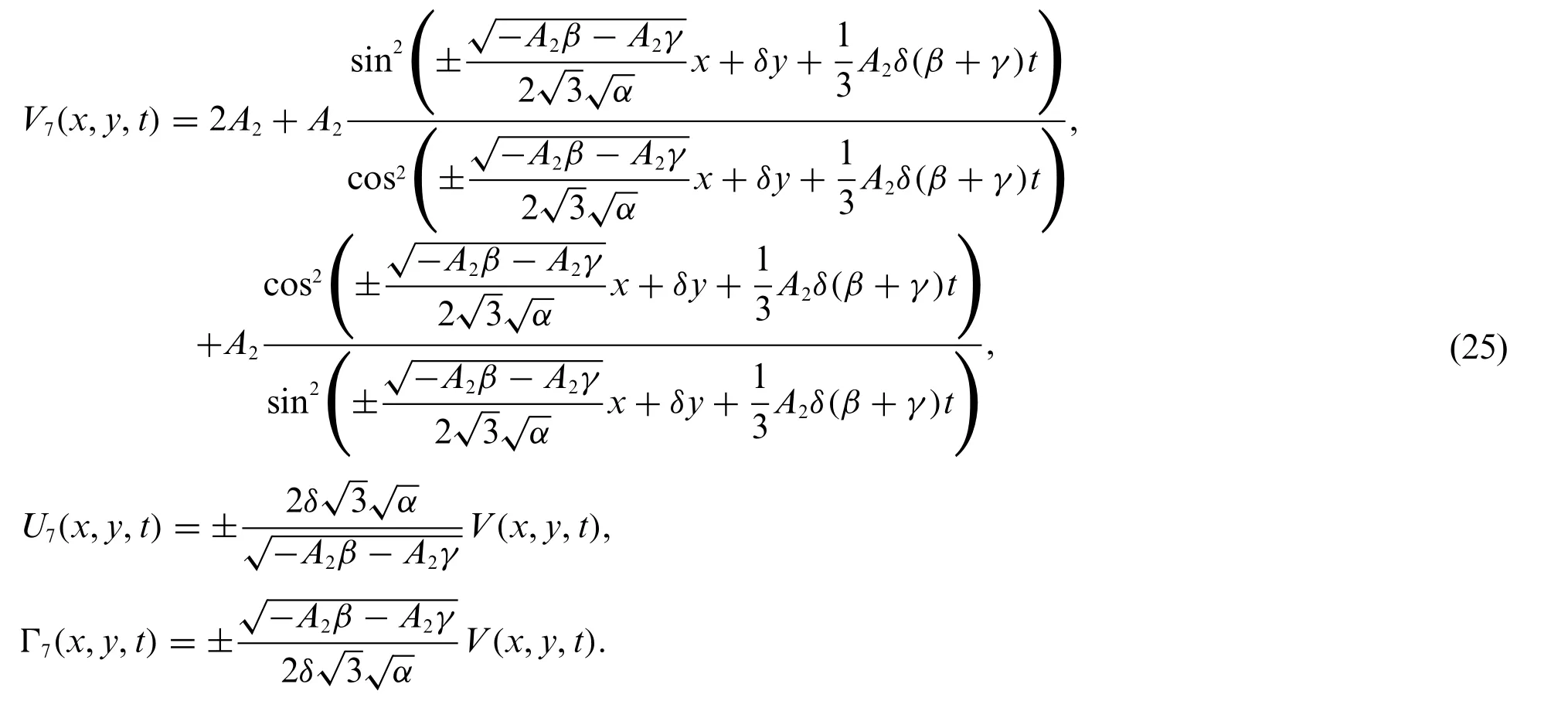
Case 4:

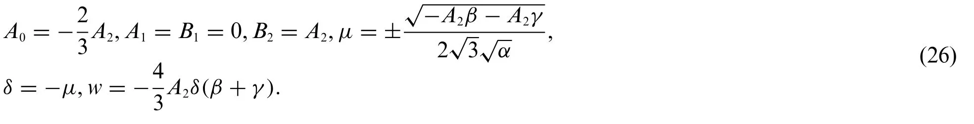
Substituting Eq.(26)into system(9)and Eq.(19)leads to the exact solutions of system(1)which are expressed as

4 Stability of the Analytical Solution

We introduce the Hamiltonian system in this section.Hamiltonian system is applied on analytical solutions to test their stability on a specific interval.The Hamiltonian system[24,25]is expressed by

whereΠindicates the momentum function.Furthermore,wpresents the wave speed andv(ζ)is the considered analytical solution.The sufficient condition for the stability is

When we apply Eqs.(28)and(29)on Eq.(18)over the rectangular domain[-20,40]×[0,1],we obtain

where the parametersA2=1.2,β=-0.5,α=2.70,andγ=-2.20.As a result,the analytical solutions are unconditionally stable.

5 Finite Difference Semi-Discretization Scheme on a Fixed Mesh

This section is devoted to study the numerical solutions of system (1) over the physical domain[a,b]×[c,d],whereaandbindicate the boundary of the domain inxdirection.Moreover,canddindicate the boundary of the domain inydirection andTedenotes a specific time.The central finite differences are utilized to establish the numerical schemes of this system.We firstly split the domain[a,b]×[c,d]into(N+1)×(M+1)discrete points as follows:

xn=a+nΔx,n=0,1,2,...,N,

ym=c+mΔy,m=0,1,2,...,M.

Here,ΔxandΔydenote the width of the sub-intervals inxandydirections,respectively.System(1) is now converted into some equations of ODEs by implementing finite differences on spatial derivatives.We keep the temporal derivative continuous.Completing this gives

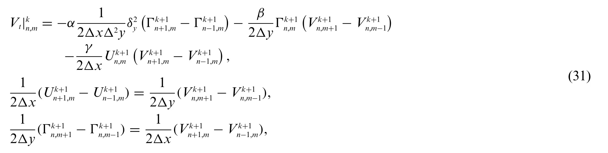
where

We compute the boundary conditions as follows:

These boundary conditions allow us to employ the fictitious points in computing the spatial derivatives at the boundaries of the domain.It is worth noting that the initial conditions are established by evaluating the exact solution att=0,as follows:

whereδ=∓A2,β,γ,αare constants.

In order to extract the numerical solutions of the considered equation,we implement the finite difference approach which depends on a standard ODE solver in FORTRAN software,DASPK solver[25].The standard backward differentiation operators are invoked to approximate the time derivatives in this solver.In addition,the Jacobian matrix of the linearised system is approximated by applying LU factorization.To have less bandwidth for this matrix,we use a unique system numbering for the unknownsV1,1,V2,1,V3,1,...,VN+1,M+1.

6 Stability of the Numerical Solution

This section investigates the stability of the numerical solution using a Fourier’s stability technique.From the second and third equations of system(8),we have

Substituting these equations into the first equation of system(1)yields

whereSince the Fourier stability approach is applied on linear equations,we linearise Eq.(34)as follows:

whereL0andL1are constants quantity defined by

The boundary conditions are ignored.Consider the point(xn,ym,tk),wherexn=nΔx,ym=mΔyandtk=kΔt.Let

plugging Eq.(36)into scheme(35)yields

Dividing both sides of the result bygives

Assume that

Then,Eq.(38)becomes

Hence,

According to the Fourier stability,the stability of the considered scheme occurs if the absolute value ofλdoes not exceed one.This constrained condition is perfectly satisfied in our analysis.It is clear from Eq.(39)that the absolute value ofλis less than one.Consequently,the numerical scheme is unconditionally stable.

7 Error Analysis

Taylor series is used in this section to examine the order of the accuracy of scheme(31).We evaluate the truncation error to obtain the order.Suppose that

wheredenotes the error,andV(xn,ym,tk+1)represent the approximation solution and the analytical solution at(xn,ym,tk+1),respectively.We now insert Eq.(41)into scheme(35)to obtain

whereis the truncation error which is expressed as

The leading terms mentioned above are known as the fundamental part of the local truncation error,and we have accepted the truth thatu(x,y,t)is the solution of the underlying system.Therefore,

The truncation error,which is generated in every step,is given byO(Δt,Δx2,Δy2).

8 Convergence of the Numerical Schemes

Now consider that a sequence of computations is carried out using given initial data,with the refinement of three meshes,so thatΔx→0,Δy→0 andΔt→0.Then,the numerical scheme is said to be convergent if,for each fixed point(x*,y*,t*)in a chosen domain[a,b]×[c,d]and[0,Te],

We have established above that the implicit schema is unconditional stability.So,we will show that the implicit schemes are unconditional convergence.Suppose that the erroreis given by

Now,satisfies the scheme (Eq.(31)) exactly,whileV(xn,ym,tk)omits the error indicated by the truncation error.

Hence by using the fact thatVy=Ux,andVx=Γyand subtraction,we have

whereis truncation error(see Eq.(42)).If we suppose that the maximum error for time step is given by

Substituting Eq.(46)into Eq.(45)yields

Since the above inequality holds for eachn=1,...,N-1 andm=1,...,M-1,we have

Since the given initial data is used we can identifyE0=0.Hence the inequality is given by

But→0 asΔx,Δy,Δt→0,then

Hence,the scheme(Eq.(31))is convergent asΔx,Δy,Δt→0.

9 Results and Discussion

In this section,we discuss the results shown in this work.We extract a distinct range of traveling wave structures of the two-dimensional Riemann problems via the generalized exponential rational function method.The obtained solutions are presented in terms of trigonometric and hyperbolic functions.We examine the stability of Eq.(18) over the rectangular domain [-20,40]×[0,1] by applying Eqs.(28)and(29)on this equation.Since Eq.(30)is positive,the exact solutions are stable with the used parameters which areA2=1.2,β=-0.5,α=2.70,andγ=-2.20.

The numerical solutions are discussed by employing the finite difference method to convert the underlying problems into the system of ODEs with keeping time derivatives continuous.Then,I solve the resulted ODEs system using the DASPK solver.This method gives reliable and powerful results.This can be clearly seen in the graphical comparisons presented in the above-mentioned figures.For instance,Figs.1 and 2 illustrate the behavior of the analytical and numerical solutions fort=5 andt=10,respectively.It can be easily observed from these figures that the solutions nearly have the same behavior.In Fig.3,the exact and numerical solutions approximately have the same behavior whent=20.Fig.4 presents the time evolution ofV(x,y,t)to the traveling wave structures(a)the analytical and (b) the numerical solutions with parameter valuesA2=1.2,β=-0.5,α=2.70,andγ=-2.20.Fig.4b also illustrates the performance of the used approaches.Moreover,Fig.5 shows acceptable performance for the used numerical technique when a massive number of meshes is used.For example,when we useN=120,the error is high.Nevertheless,the numerical solutions approximately approach the exact solution (blue line) forN=3000.The stability of the numerical results is investigated using the Fourier technique.Since|λ| ≤1 in Eq.(40),the numerical scheme is unconditionally stable.Furthermore,the accuracy of the numerical scheme is ofO(Δt,Δx2,Δy2).

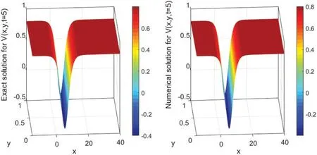
Figure 1:Surface plot of V(x,y,t)presenting the analytical(left)and the numerical(right)solutions’evolution in time t=5 using N=3000 with Δx=0.02 and M=100 with Δy=0.01.The parameter values are A2=1.2,β=-0.5,α=2.70,and γ=-2.20

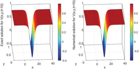
Figure 2:Surface plot of V(x,y,t)presenting the analytical(left)and the numerical(right)solutions’evolution in time t=10 using N=3000 with Δx=0.02 and M=100 with Δy=0.01.The parameter values are A2=1.2,β=-0.5,α=2.70,and γ=-2.20

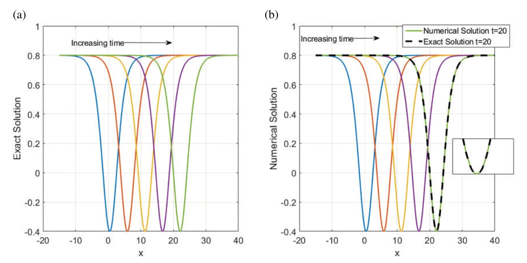
Figure 4:Time evolution of V(x,y,t)to the traveling wave structures(a)the analytical and(b)the numerical solutions with parameter values A2=1.2,β=-0.5,α=2.70,and γ=-2.20.(b) also illustrates the performance of the used approaches

Table 1 illustratesL2errors and the CPU times taken to reacht=20.The error decreases for largeNbut the method takes more time to give a small error.We begin withN=120,Δx=0.50 andΔy=0.01.TheL2error stands at 5.37×10-4during 0.74 min.When we useN=3000 withΔx=0.02 andΔy=0.01,theL2error dramatically decays and stands at 1.073×10-6during 20.63 min.Fig.6 shows the decay in theL2error asNincreases.

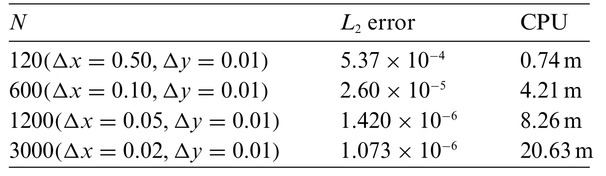
Table 1: L2 errors and CPU times taken to arrive at t=20

Figure 5:Presents a comparison of the numerical results of Eq.(31)at t=20 for increasing N of the spatial variable x.The solid blue line shows the exact solution Eq.(12).The parameter values are A2=1.2,β=-0.5,α=2.70,and γ=-2.20.The insets present zoomed-in wave characteristics

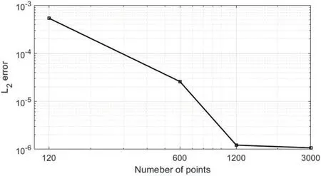
Figure 6:Illustrating L2 errors presenting in Table 1

10 Conclusion

We have favorably implemented an accurate finite difference method on a uniform mesh and the generalized exponential rational function method for the two-dimensional Riemann problems.The main advantage of the results is to show the traveling wave structures and prove their accuracy using numerical methods.By comparing the exact solutions using the generalized exponential rational function method with those from the numerical scheme,it was said that the numerical results are almost identical to the analytical results.It is well known that the numerical scheme is stable and allows a meaningful reduction in memory requirements.Using a fine mesh in both spatial variablesxandypermits us to resolve the wave-like structures.We can conclude that the used methods can be efficiently applied to more nonlinear evolution models to construct their exact and numerical solutions.

Funding Statement:The author received no specific funding for this study.

Conflicts of Interest:The author declares that they have no conflicts of interest to report regarding the present study.