Numerical modeling and experimental investigation of a two-phase sink vortex and its fluid–solid vibration characteristics

Zichao YIN, Yesha NI, Lin LI, Tong WANG, Jiafeng WU, Zhe LI, Dapeng TAN

Research Article

Numerical modeling and experimental investigation of a two-phase sink vortex and its fluid–solid vibration characteristics

1College of Mechanical Engineering, Zhejiang University of Technology, Hangzhou 310014, China2State Key Laboratory of Fluid Power and Mechatronic Systems, Zhejiang University, Hangzhou 310058, China

A sink vortex is a common physical phenomenon in continuous casting, chemical extraction, water conservancy, and other industrial processes, and often causes damage and loss in production. Therefore, the real-time monitoring of the sink vortex state is important for improving industrial production efficiency. However, its suction-extraction phenomenon and shock vibration characteristics in the course of its formation are complex mechanical dynamic factors for flow field state monitoring. To address this issue, we set up a multi-physics model using the level set method (LSM) for a free sink vortex to study the two-phase interaction mechanism. Then, a fluid–solid coupling dynamic model was deduced to investigate the shock vibration characteristics and reveal the transition mechanism of the critical flow state. The numerical results show that the coupling energy shock induces a pressure oscillation phenomenon, which appears to be a transient enhancement of vibration at the vortex penetration state. The central part of the transient enhancement signal is a high-frequency signal. Based on the dynamic coupling model, an experimental observation platform was established to verify the accuracy of the numerical results. The water-model experiment results were accordant with the numerical results. The above results provide a reference for fluid state recognition and active vortex control for industrial monitoring systems, such as those in aerospace pipe transport, hydropower generation, and microfluidic devices.

Free sink vortex; Fluid–solid coupling; Level set method (LSM); Multi-physics model; Vibration characteristics

1 Introduction

As the liquid drains out from the bottom of a limited-space container, a two-phase sink vortex with a free surface is formed in the anaphase of the drainage, due to the effect of gravity, Coriolis force, and other external disturbances (Jeong, 2012). A free sink vortex is found in a wide range of engineering processes, such as continuous casting, chemical extraction and separation, rocket fuel supply, and hydropower generation. Its scale is related to the initial disturbance velocity, container geometry, and surface roughness (Tan et al., 2013, 2018, 2020). However, the appearance of a free sink vortex is always undesirable, as it can easily reduce production quality and the energy utilization rate, and may cause enormous economic losses (Lu et al., 2020). For example, in continuous casting, vortex suction affects the purity of the molten steel and reduces the quality, leading to industrial accidents (Li et al., 2020). During tidal power plant operation, a surface vortex can induce irregular loads, affect turbine performance, and increase the risk of damage. From a safety viewpoint, the gas entrainment phenomenon of a free surface vortex is an essential issue in a rocket fuel system. Given these issues, reliable and accurate monitoring of the flow field is critically important for some industrial processes in relation to the sink vortex. However, under some harsh working conditions, such as high temperature, confined space, or substantial magnetic interference, the flow field is often prevented from being directly observed by video devices (Li et al., 2023a). Therefore, an indirect monitoring method based on fluid-structure interaction analysis and vibration signal identification is needed to reveal the dynamic properties of the flow field of a free sink vortex. The key technologies require numerical modeling and experimental studies of two-phase free sink vortexes and their fluid–solid shock vibration characteristics.

Although a free sink vortex is a common natural phenomenon, it is a complex turbulent mechanical problem. There are no mature theoretical models for quantitative analysis of the genesis and motion law (Sleiti, 2020). It can be studied only by suppositions or combined with experiments to obtain partial features. Related studies (Mikota and Mikota, 2020) suggested that a strong shock wave vibration exists during the formation and suction process of a vortex. The generation of shock wave vibration is closely related to the critical state transition of the vortex, which is the result of internal turbulent energy accumulation and release. The evolution of the two-phase interface is often highly nonlinear due to the suction of the sink vortex and the viscous friction at the interface (Sangalli and Braun, 2020). Numerical simulation and experimental research on two-phase sink vortexes and their fluid‍–‍solid coupling vibration face significant challenges. In this paper, we describe the formation and coupling mechanism of a two-phase sink vortex and then reveal the relationship between the critical penetration state and fluid–solid shock vibration characteristics.

There have been many numerical and experimental studies of the factors contributing to the formation of a sink vortex. Koria and Kanth (1994) verified experimentally that the drainage of two-phase fluids, due to their different physical properties, is not synchronized in the suction process of a vortex. The critical problem is that the dense friction effect at the two-phase interface causes the motion laws to take on nonlinear characteristics. Lundgren (1985) researched the formation mechanism of a free sink vortex, based on an axisymmetric model and the Ekman layer theory. He concluded that the nonlinear drainage in the vortex formation process was similar to the non-viscous flow in the Ekman boundary layer. Andersen et al. (2003, 2006) confirmed that circumferential velocity is the main reason for the formation of vortexes, based on the Ekman layer theory. Their experimental results showed that the vortex formation process produces a shock vibration with a sharp sound. Cristofano et al. (2016) investigated bathtub vortexes using particle image velocimetry (PIV) experiments, and showed evidence of a clear dependence on Reynolds number and distance from the outlet hole. Li et al. (2016) showed that the Coriolis force had little effect on vortex formation, and suggested the initial tangential disturbance was the main factor. Turkyilmazoglu (2011, 2018) described the exact solutions related to rotating incompressible fluid flows over surfaces formed by the superposition of a uniform source and an irrotational vortex. Based on the Helmholtz equation, Tan et al. (2016, 2019) presented a solution to acquire the critical penetration condition, and discussed the Ekman boundary layer. However, there have been few studies of the two-phase coupling phenomenon of a sink vortex. Given the different physical properties of mediums, vortex suction can cause intense motion of the phase components and appear to have highly nonlinear characteristics. This will cause a turbulent energy transition in the vortex formation process and induce fluid–solid shock vibration.

It can be inferred from the above that current research on vortex vibration crosses the disciplines of solid mechanics, fluid mechanics, and vibration dynamics, and focuses mainly on the contributing factors and a single-phase. The coupling formation mechanism of a two-phase sink vortex and the transient vibration dynamic characteristics have not been precisely defined. The features of fluid–solid coupling vibration indicate that the fluids act on the wall under a particular driving force and appear nonlinear with variation of the driving force. In the process of formation of a free sink vortex, the nonlinear excitation of two-phase fluids acts on the thin wall and causes different vibration features to appear. In our previous studies, we simulated fluid–solid coupling vibration based on the Flügge equations and discrete wavelet transform to reveal the vibration wave transition mechanism, but the results lacked supporting experimental data (Li et al., 2021, 2023d). Therefore, it was necessary to propose a fast calculation and stable fluid-structure coupling model and a vibration signal processing method to establish an experimental platform and demonstrate its enhanced application potential in a real-time field anti-vortex strategy.

In this paper, we present a numerical modeling method for a two-phase sink vortex to investigate the coupling formation mechanism, based on the critical penetration characteristics. A single-phase-based fluid–solid coupling dynamic model oriented to vortex-induced vibration was set up to study the shock vibration characteristics and identify the state of the sink vortex. The corresponding technical route was as follows: (1) Based on the level set method (LSM), the evolution process of a sink vortex two-phase interface was tracked. (2) A fluid–solid coupling dynamic model was set up to investigate the shock vibration characteristics and reveal the transition mechanism of the critical flow state. (3) An experimental observation platform was established to verify the critical penetration vibration attributes of the numerical results.

This paper is organized as follows: In Section 2, the fluid-structure coupling dynamics model is described, and an interface tracking method is proposed. In Section 3, the numerical model and boundary conditions of the two-phase sink vortex are given. In Section 4, the numerical results after coupling are analyzed. In Section 5, we describe the fluid–solid vibration experiments. In Section 6, we draw conclusions from the results.

2 Mathematical model and solution method

2.1 Multiphase flow coupling model

The research objectives of the sink vortex in this paper relate mainly to the two-phase flow coupling mechanism, interface tracking, and its fluid–solid coupling vibration. The two-phase fluid contains air and water that exist in a finite physical space (Tan et al., 2017). The conservation equation of mass and momentum is as follows:

whereis the mixture average velocity,is the gravitational acceleration,is the fluid pressure,is the fluid density,is the fluid viscosity,is the time, andis the surface tension force per unit volume.

The LSM is widely used in research on multiphase flow and can solve the dynamic tracking problem of a mobile phase interface. Luo et al. (2015) improved the mass conservation LSM for the detailed numerical simulation of liquid atomization. Balcázar et al. (2015) used the conservative LSM to study single and multi-bubble buoyancy-driven motions numerically. Kinzel et al. (2018) proposed an LSM suitable for compressible and incompressible multiphase flows. The LSMs applied in the above research provide an essential reference for studying the evolution mechanism and real-time tracking method for a two-phase interface.

The LSM smooth function(,) describes the interface between the different stages of the flow field (Kaiser et al., 2020). It represents the distance from each point to the interface. The zero level set function on the interface boundary can be defined as

whereis satisfied as:

Then, the multiphase flow field is divided into two different domains:

where1is described as the dispersed phase, and2as the continuous phase.is the interface of the two regions. The curvature of the interfacecan be expressed as

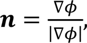
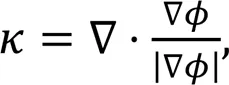
whereis the normal vector of the interface.

Sinceis a continuum surface, the fluid densityand viscosityat the boundary area can be described as

where() is a Heaviside step function, and the subscripts 1 and 2 represent the primary and secondary phases of the multiphase flow system, respectively. In the process of LSM iteration, even after a time step, the level set function is no longer an accurate distance function. One way to resolve this difficulty is to re-initializeat each time step into the exact distance function from the evolved frontby solving the following equations:

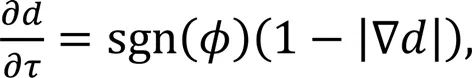
whereis virtual time,is the distance function, and sgn() is a sign function. The whole LSM solution process first needs discretization and projection in space, so that the velocity field has no divergence. Then the time is discretized, and finally the reconstructed() is initialized to further improve the accuracy of the numerical solution. In addition, the two-phase spatial discretization solution is given in Section S1 of the electronic supplementary materials (ESM), including the step of high-order essentially non-oscilatory (ENO) method (Cao et al., 2022).

The formation of a free surface vortex constitutes a complex and unsteady flow process, characterized by highly nonlinear behavior. When an initial disturbance exists in the flow field, it evolves into a fully developed turbulent state. The realizable-model, a classical turbulence model, has gained traction in engineering applications due to its dependable robustness and stability (Morales et al., 2013). This model incorporates variables related to rotating velocity and curvature, resulting in improved computational accuracy for flow fields exhibiting intense flow line curvature, surface vortexes, and swirling flow (Li et al., 2021). Consequently, the realizable-model has been adopted to track turbulent vortex motions:

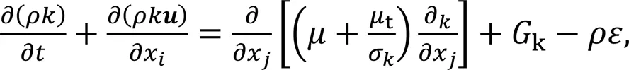
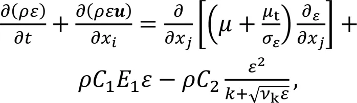
wherexandxrepresent two different spatial directions,is the turbulent kinetic energy, andis the dissipation rate.σandσare the Prandtl numbers ofand, respectively.1represents the time mean strain rate tensor modulus,kis the kinematic viscosity,kis the turbulent kinetic energy, andtis the turbulent viscosity coefficient, which can be expressed ast=ρCk2/. The empirical parameters in the model are as follows:1=1.44,2=1.92,σ=1.0, andσ=1.3.

Within the aforementioned turbulent model,Crepresents a crucial variable int. It functions as a specialized expression involving parameters such as swirling velocity, time-averaged strain, turbulence intensity, and angular speed (Chen et al., 2015). When subjected to significant time-averaged strain, the model effectively adheres to the restraining conditions of Reynolds stress, ensuring a flow state that aligns more accurately with the regularities of turbulent physics. The simulated multiphase vortex exhibits characteristics of a highly nonlinear turbulent viscous vortex (Li et al., 2021). The complexity of the interphase viscidity resistance causes the functionCto vary with the vortex evolution process.

2.2 Fluid–solid coupling vibration model

The interaction between the fluid and the wall surface is achieved through the contact condition of the interface, and the contact stress–strain relationship is described by:

whereσ,σ, andσare the axial, circumferential, and radial contact stresses of the container wall, respectively;is Young's modulus of the wall material;is Poisson's ratio;ε,ε, andεare the axial, circumferential, and radial contact strains of the wall, respectively. According to the strain displacement relation contained in the geometric equation, the axial stress can be derived by combining the above equations:

whereuanduare the axial and radial flow speeds, respectively. Based on the above equations, the relationship between the stress and velocity of the axial equation can be obtained according to the constitutive relation of the container surface mechanics:

whereis the thickness of the pipeline, andis the inner diameter of the pipe. Generally, the wall thickness is less than inner diameter, so it can be supposed that the velocity on the inner wall is equal to that on the outer wall, i.e.u|=R+δ=u|=R. According to this hypothesis, Eq. (18) can be simplified to

After further simplification of the axial stress, we obtain

Taking the derivative of Eq. (20) to time, the relationship between the axial stress and the velocity of the container is

In Eq. (21):

Based on the above hypothesis, the fluid–solid coupling vibration 4-equation model can be obtained by ignoring the radial inertial force, centrifugal force, and Coriolis force in the contact process:

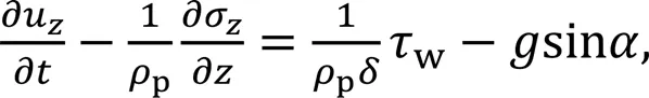
Eqs. (24)‍–‍(27) are the fluid axial motion equation, fluid continuity equation, structure axial motion equation, and structure physical constitutive equation, respectively.fis the average velocity of flow,pis the pipeline density,fis the fluid density of the mixed phase,is the mean pressure of the liquid,fis the volume modulus of the fluid,wis the friction between the fluid and the wall surface, andis the dip angle of the pipeline.

3 Implementation of free sink vortex model

3.1 Mechanical model and boundary conditions

A physical model was set up to investigate the mechanical characteristics of the sink vortex (Fig. 1a). The container in the physical model had an upper diameter of 120 mm, a bottom diameter of 88 mm, and a height of 130 mm. The two-phase fluids in the container consisted of liquid (at the bottom, 91 mm) and air (at the top, 39 mm). Based on the dynamic characteristics of the vortex, a mechanical and dynamic model of a multiphase fluid was set up (Fig. 1b). The model was simulated using COMSOL Multiphysics 5.6, and the tetrahedron non-structure mesh scheme was used to model the calculation region, especially the refined mesh at the drainage pipe. The physical features and boundary conditions are listed in Table 1.

Fig. 1 Mechanical model of fluid–solid coupling vibration: (a) physical model; (b) mesh grid and boundary conditions

Table 1 Boundary conditions of the mechanical model

The finite volume method discretizes the control equations to ensure strict fluid mass conservation. Since the multiphase sink vortex simulation belongs to an unsteady state process, phase and phase variation in multiphase coupling are complex. The PISO (pressure implicit with the splitting of operators) algorithm was adopted to deal with the pressure–velocity coupling and ensure convergence efficiency (Yuan et al., 2016).

3.2 Solid model and boundary conditions

The fluid–solid vibration model was to set a solid constraint on the fluid model. The flow would induce shock vibration on the wall during drainage, and the effect could be analyzed by detecting the vibration of the inner wall. This demands a solid inner wall mesh, and the mesh division needs to be denser due to the nonlinear impact of the sink vortex (Wang et al., 2023). The physical features and boundary conditions are listed in Table 2.

The model focuses on coupling the fluid domain and the solid domain, and considers the shock vibration generated by the fluids acting on the wall surface. The pressure at the outlet in the fluid model is1, and that at the inner wall in the solid model is2(Fig. 1a). The simulation considers the coupling of fluid and solid, and the numerical equation completes the data exchange from1to2of the coupling wall. During the formation and evolution of the sink vortex, the value of1changes constantly and affects the deformation status of the inner wall (Sam et al., 2018). Therefore, the dynamic vibration characteristics of the sink vortex can be obtained by analyzing the displacement variation features of the solid wall.

Table 2 Boundary conditions of the solid model

Based on the above hypothesis, the displacement data of a point on the solid model can be obtained, and the vibration acceleration data can be obtained by two derivations of the time. In this study, we selected acrylic plastic with a small Young's modulus that could obtain large displacement as the material. The simulation applies the fluid–solid method only to capture the shock vibration characteristics and cannot consider the influence of the temperature field on the solid structure. As the fluid impact affects the wall, the wall surface deformation is more extensive, and the shock vibration is more prominent. The physical properties of the material are shown in Table 3 (Ge et al., 2018).

Table 3 Material attributes of the coupling model

3.3 Validation of the mechanical model

The model data with=14 mm were used as an example to verify the mechanical model (Fig. 2). A weighing instrument was placed on each side of the support plate to verify the volume fraction of the drainage process. The water content was obtained indirectly from the mass variation. In Fig. 2, the time interval in the simulation was 0.2 s, and in the experiment, the time interval was 1 s due to the quick drainage process.

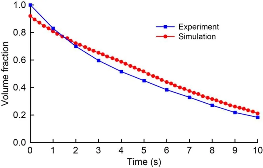
Fig. 2 Volume fraction of the drainage process

As the drainage progresses, the volume fraction data show a decrease in the rate of decline. Some air drains from the outlet instead of water with the generation of the sink vortex, which leads to a decrease in the drop rate of the volume fraction. In the simulation, it is difficult to form a vortex at the outlet because of the lack of Coriolis force. Therefore, a swirling wall was used to disturb the flow field to ensure the formation of a sink vortex. This results in a lower central area of the liquid level in the early stage, and leads to vortex penetration in advance.

The volume fraction in the simulation was obtained by monitoring the area from the bottom of the container to the initial liquid level height. Due to the gas phase in the center of the liquid level, the volume fraction in the simulation was less than 1. However, the volume fraction in the experiment was obtained indirectly by detecting the fluid quality, which led to the difference in the initial value between simulation and experiment. With the drainage process, the liquid above the initial liquid level in the simulation gradually decreases, which to some extent compensates the drainage fluid and reduces the rate of decline in the volume fraction. In addition, the initial disturbance in the simulation was more significant than in the experiment, so the vortex generation occurred earlier, and the volume fraction dropped more slowly. The decline rate of data was almost uniform due to the formation of the sink vortex in the anaphase of the drainage. The mesh schemes have an important influence on the accuracy of numerical solution. In order to achieve a balance between accuracy and efficiency, the mesh independence study is provided in Section S2 of the ESM.

4 Numerical results and discussion

4.1 Streamline and volume fraction

A sink vortex often occurs in many industrial processes and is associated with significant damage (Zheng et al., 2021). For example, in the anaphase of continuous casting ladle teeming, a sink vortex can suck the liquid slag into the tundish and have negative effects on the purity of molten steel (Wang et al., 2021). A similar situation often appears in chemical extraction and water conservancy (Fan et al., 2021). In these situations, the vortex penetration state is critical in sucking upper impurities. Therefore, in this study we focused on the two-phase suction mechanism and the critical penetration condition of the sink vortex. Based on the dynamic mechanical model, the 3D fraction streamline profiles and volume fractions of the critical penetrating state with different nozzle diameters were obtained (Fig. 3).

Fig. 3 shows several typical cases in which=4, 8, and 14 mm. Each group of comparisons is divided into a gas‍–‍liquid two-phase distribution diagram and a two-phase streamline coupling diagram. The figure shows that the phenomenon of multiphase coupling can be observed, and the coupling strength increases with the flow rate at the outlet. After the sink vortex penetrates the outlet, the two-phase coupling phenomenon of water and air appears in the container and shows a highly nonlinear characteristic. The impurities mix into the fluid and enter the outlet via a descending spiral flow. In Fig. 3d, it is difficult for the pollutants to flow into the outlet due to the lower vortex intensity. In contrast, in Fig. 3f, in the vortex with a higher rotating velocity, the impurities could more easily enter the outlet and had a more extensive volume fraction. The formed vortex scale would be more significant with increasing diameter of the outlet. Under the condition of vast liquid inside a container, it will result in a penetrating phenomenon that should be avoided in many industrial processes. In the case where=4 mm, the formed vortex was much smaller than the others, as required in some production processes.

Fig. 3 Volume fraction profile and streamline profiles of vortex penetration: (a) volume fraction profile in d=4 mm case; (b) volume fraction profile in d=8 mm case; (c) volume fraction profile in d=14 mm case; (d) streamline profile in d=4 mm case; (e) streamline profile in d=8 mm case; (f) streamline profile in d=14 mm case

The time-varied waves of volume fractions were obtained (Fig. 4) to perform further research on the volume fraction profiles in relation to the nozzle diameters. The results show that: (1) With increasing nozzle diameter, the descent rate of the water fraction increases, and the volume fraction of14 mm can reduce to 0. (2) The volume fraction of4 mm only reduces to less than 0.7, proving that a lower outlet flux can effectively restrain the quantity. (3) As the vortex is penetrating, the rate of decline of the volume fraction decreases. In general, the flow flux controls the intensity of the formed sink vortex. In satisfying the requirements of the industrial processes, the nozzle diameter of the drainage pipe should be reduced.

Fig. 4 Time-varied waves of volume fractions for different nozzle diameters

4.2 Pressure profiles of vortex formation process

The total pressure at the outlet can reflect the kinetic energy characteristics of a sink vortex (Li et al., 2023b, 2023c). Fig. 5 shows the variation of the total pressure in the drainage process. The total pressure in the figure is given by reference to standard atmospheric pressure. As the total mass of the container decreases due to drainage, the total pressure trends downward. The average total pressure was the highest at=4 mm, i.e., the downward trend of the total pressure was the slowest. The flux was closely related to the total pressure. In contrast, the average total pressure was the lowest at=14 mm, the curve decreased more slowly with the draining process, and the total pressure decreased faster before vortex penetration. The total pressure gradually reduced with the fluid flowing out of the outlet. In the anaphase of drainage, due to the generation of the sink vortex, the gas was sucked into the liquid, and caused the flux to be reduced, wherein the trend of total pressure stabilized. In particular, the total pressures at=12 and 14 mm tended to be balanced at 10 s, caused by penetration of the outlet by the vortex. After that, impurities and air entered the outlet, and the variation curve decreased slowly, which was similar to the change of the volume fraction.

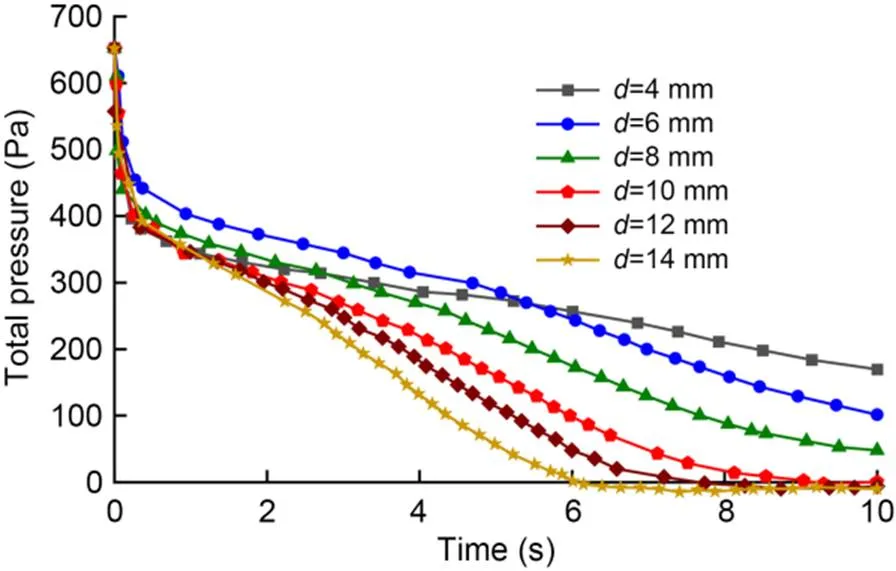
Fig. 5 Pressure profiles of the vortex formation process

The two-phase coupling of the sink vortex produces non-periodic energy diffusion, which can cause shock vibration to the drain tube (Lin et al., 2022). This leads to obvious oscillation of the total pressure curve in the drain anaphase. The total pressure curve at=14 mm oscillated first due to the sink vortex penetrating the outlet. The larger the outlet, the earlier the penetration by the sink vortex. The sink vortex was generated and penetrated the outlet late because of the small flux. Therefore, at=4 and 6 mm the curve had no apparent oscillation. A noteworthy phenomenon is the negative pressure implied during vortex formation. The value below the reference atmospheric pressure presented in Fig. 5 may be affected by two factors: (1) The vortex has aperiodic energy diffusion in the penetration stage. The wall surface produces strain under the fluid–solid coupling effect, making the drainage diameter expand and causing the local pressure to decrease. This phenomenon is more evident in the large diameter pipeline because the greater flow has a more severe impact on the wall surface, making the structural deformation more obvious. (2) A tetrahedron non-structure mesh scheme was used to model the calculation region, especially the refined mesh at the drainage pipe. There is a large-scale difference between the meshes in the drainage pipe and those in the container. Numerical calculation accumulates significant errors when pressure data are transmitted between meshes of different scales, making the pressure here lower than the reference pressure point. Based on the above analysis, we conclude that vortex penetration causes the pressure curve oscillation. This characteristic provides technical support for vibration-based industrial systems, and the formation of the sink vortex can be predicted.

4.3 Frequency domain of the vibration signal

Through fast Fourier transform (FFT), the frequency-domain distribution of the vibration signal is obtained during the drainage process (Fig. 6). The abscissa is the signal frequency and the ordinate is the acceleration amplitude of the vibration signal. With increasing outlet diameter, the oscillation times of the vibration signal decrease and the peak value gradually declines. The main reason is the decrease in accuracy caused by a small number of model data points with a large outlet diameter. The sampling frequency was 100 Hz in the four simulations, and the larger outlet models had a higher flux and longer drainage time, resulting in fewer data points in the whole drain process. For example, the=8 mm model had a total of 15960 data points, while the=14 mm model had only 7460, fewer than half of the former. Therefore, the frequency analysis at=8 mm was closer to the actual situation than that of the other three experiments. In addition, the low-frequency signal was weaker in the whole drain process, while the high-frequency signal was stronger. The amplitude of the frequency signal below 200 Hz in the model at8 mm was less than 2×10-5(m/s2)2, and its amplitude in the range of 200–300 Hz increased gradually. In the high-frequency signal, the signal amplitudes of many bands were higher than 3×10-5(m/s2)2.

However, the frequency-domain analysis of the vibration signal in the whole drainage process could not prevent vortex formation. Frequency-domain analysis at different stages of the process of vortex formation was conducted to study the critical penetration attribute. The frequency-domain data at8 mm of four time periods were extracted (Fig. 7).

In the first 10 s, the sink vortex was formed far away from the outlet. After 10 s, it gradually approached the outlet, and completely penetrated the outlet in 16 s. Fig. 7a (0–5 s) is very similar to Fig. 7b (0–10 s). This indicates that the flow characteristics in the two time periods were almost identical. In the range of 11–12 s, the vortex developed to its maximum scale and approached the outlet, causing the vibration signal to increase sharply. This was evident in the high-frequency bands, particularly in Fig. 7c. After that, the low-frequency signal (0–150 Hz) showed no apparent variation and the frequency signal (150–350 Hz) had increased by 1.5 times, while the high-frequency signal (350–500 Hz) nearly doubled (Fig. 7d). This suggests that the amplitude of the high-frequency signal is an important feature for sink vortex identification and precaution.

Fig. 6 Frequency-domain profiles of the vibration signal: (a) d=8 mm; (b) d=10 mm; (c) d=12 mm; (d) d=14 mm

Fig. 7 Frequency-domain profiles during various time periods (d=8 mm): (a) 0–5 s; (b) 0–10 s; (c) 0–12 s; (d) 0–14 s

5 Fluid–solid vibration experiment

5.1 Experimental platform construction

To verify the fluid–solid mechanical dynamic model in this paper, an experimental platform of a sink vortex was set up based on the similarity second law of fluid mechanics (Pan et al., 2020), as shown in Fig. 8a. The experimental device consisted of a perspex container with a drainage pipe. Fluid transport and circulation of the vortex formation process were realized through the fluid circulation module. To achieve accuracy, factors influencing the experimental results should be controlled as much as possible. Under the experimental conditions, because the liquid viscosity varies with temperature, the viscosity of the fluid medium is an important parameter to show the characteristics of fluid flow (Lyu et al., 2023). The viscosity coefficient also plays a crucial role in the turbulent kinetic energy and dissipation rate transport equation, so temperature should be maintained at a stable value. The experiment was conducted at a temperature of 20 ℃ to ensure a stable fluid viscosity coefficient (Ji et al., 2012).

Fig. 8 Experimental platform of vortex shock vibration (a) and installation position of integrated circuits piezoelectric (ICP) vibrating sensor (b). 1: container; 2: ICP vibrating sensor; 3: current adapter; 4: data acquisition card; 5: computer; 6: stainless-steel pump

When a sink vortex is formed in the anaphase of drainage, it will induce a series of shock vibrations on the wall. Through the vibration analysis real-time acquisition system, the vortex-induced vibration was analyzed, and vibration analysis data acquisition, conversion, processing, and other functions were achieved. The signal was received by the vibration sensor (Fig. 8b) and passed to the current adapter through the signal line. Then, it was transmitted to the computer for signal processing by a data acquisition card. The drain change was achieved by replacing the drain outlet under the bucket. The experiment was divided into three parts, and considered three different nozzle diameters.

5.2 Experimental results and discussion

Based on the sink vortex shock vibration detecting platform, the amplitudes of the shock vibration are shown in Fig. 9. The horizontal ordinate is the time, and the vertical ordinate is the acceleration amplitude of the vibration signal. The drainage process from the beginning to the process of penetration can be detected. The vibration of each group was significantly higher during a certain period of time than that during other periods for the same group. This time corresponds to the moment that the vortex in the respective experiments penetrated the drainage pipe. It can be seen that the sink vortex at=14 mm penetrated the drainage outlet first. With the reduction of nozzle diameter, the vortex penetrated the outlet later. In the prophase of experiments, there was a small vibration that represented the generation and evolution of the vortex. As the vibration amplitude reached its maximum, the vortex penetrated the drainage hole.

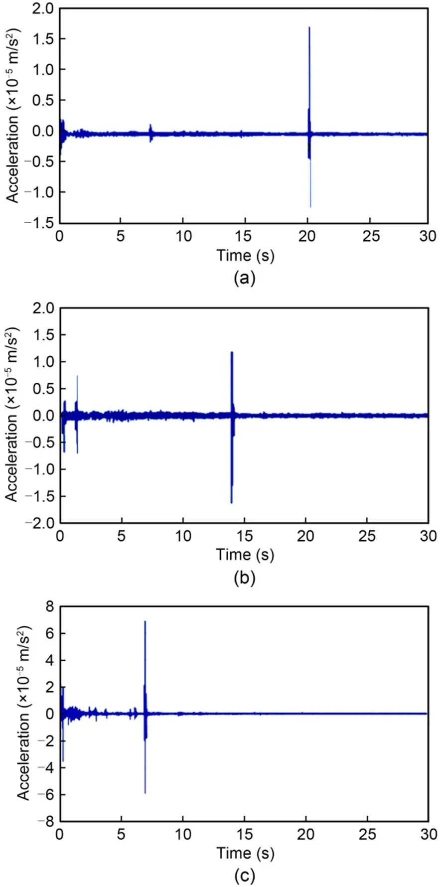
Fig. 9 Shock vibration amplitudes with different outlet diameters: (a) d=6 mm; (b) d=10 mm; (c) d=14 mm

To clearly observe the vibration characteristics of the penetration moment, the partial vibration data of experiments at the critical penetration were extracted (Fig. 10). A maximum apparent vibration attribute was observed, indicating that the vortex had passed through the drain hole. Before this, the vibration signal was stable, but then increased with the penetration process. As the energy of the sink vortex was released, the vibration signal decreased quickly. Moreover, when the drainage diameter was larger, the vibration intensity was increased. In particular, the vibration intensity at=14 mm was much higher than those of other outlet diameters. Although the maximum vibration intensity at=10 mm was not as high as that of=6 mm, the whole vibration energy at=10 mm was still greater. In general, the distortion vibration attribute of the critical penetration process provides a useful guide for relevant industrial monitoring systems. Based on a similar distortion attribute, an early warning during industrial processes could be realized, enabling the avoidance of major economic losses.

Based on the shock vibration experiment platform of the sink vortex, the spectrum attributes of the shock vibration are shown in Fig. 11. The left figure shows the vibration frequency domain of each diameter (6, 10, and 14 mm) from the beginning to the period in which the vortex is about to penetrate the outlet (Figs. 11a1, 11b1, and 11c1). The right figure shows the spectrum attributes of the whole drainage process (Figs. 11a2, 11b2, and 11c2). The phenomenon of high-frequency signal enhancement is apparent during the whole vortex penetration process. Another observation is that there is a significant positive correlation between the rising proportion of high-frequency signal and the outlet diameter. This indicates that the coupling strength of gas–liquid increases with increasing outlet diameter. The numerical calculation results in Fig. 7 are in accordance with the experimental results, and provide theoretical support for vortex prevention in industrial production.

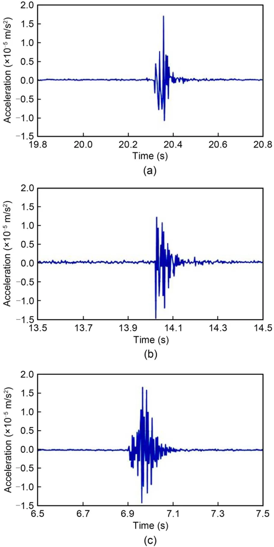
Fig. 10 Shock vibration amplitudes with different outlet diameters: (a) d=6 mm; (b) d=10 mm; (c) d=14 mm

The vibration (=14 mm) time-domain data in the simulation and experiment are compared in Fig. 12, in which the simulation data are shown in dotted line and the experimental data in solid line. Both sets of data peak at about 7 s, which is during the period of vortex penetration. The vibration duration in simulation was more significant than that in the water experiment. The simulation data begin to oscillate significantly from 5 s and peak at 7 s. However, the experiment shows that the peak was reached only in 7 s, and then the vibration disappeared. This indicates that the time from the formation of the vortex to its penetration in the simulation was longer than that in the actual situation. Before vortex penetration, multiple bubbles appeared continuously at the outlet in the simulation due to the initial disturbance and turbulence model. This process lasted for 2 s in the simulation, but passed quickly in the experiment. This process caused noise to appear in the simulation vibration signal. Despite this difference between simulation and experiment, one common effect was that the sink vortex caused shock vibration in the penetration process. This provides a useful reference for vibration detection systems.

Fig. 11 Shock vibration frequency-domain signal at different outlet diameters: (a) d=6 mm; (b) d=10 mm; (c) d=14 mm

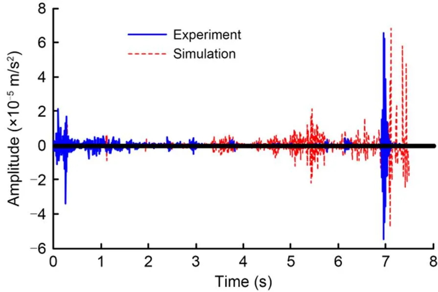
Fig. 12 Vortex shock vibration time-domain signal (d=14 mm)

The vibration (=14 mm) frequency-domain data in the simulation and experiment were obtained by FFT (Fig. 13). The sampling frequency of the water-model investigation was 1000 Hz, and the collected data were processed to 100 Hz for ease of comparison. Therefore, the highest sampling frequency of both simulation and experiment was set to 50 Hz. When the frequency-domain characters of simulation and experiment were similar, the low-frequency signal was weak while the high-frequency signal was relatively intense. In the water-model experiment, the signal around 42 Hz was significantly enhanced. In general, the frequency-domain signal characteristics were roughly similar, and the differences between them were slight. This is a reflection of the fact that a simulation can at best be only a close representation of an actual experiment. However, the enhancement of the high-frequency signal before vortex penetration is a more noteworthy phenomenon. This characteristic could be applied to detect the penetration of a sink vortex in steel continuous casting and chemical extraction, and we hope our research results can offer a universal reference for fluid state recognition in these industrial processes.

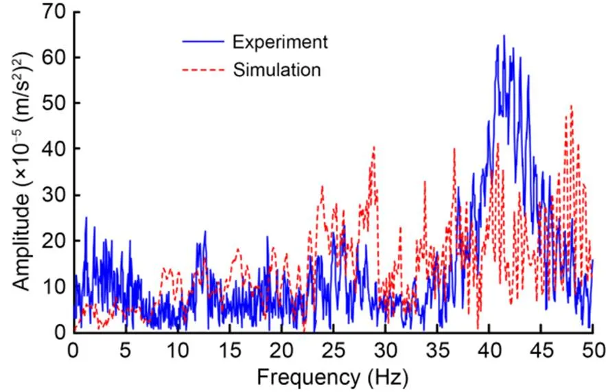
Fig. 13 Vortex shock vibration frequency-domain signal (d=14 mm)

6 Conclusions

Flow field state monitoring of the sink vortex is of vital significance for industrial processes, including metallurgic pouring, aerospace detection, and chemical extraction. It can effectively improve product quality and energy efficiency. In this paper, we have presented a method for modeling a two-phase vortex coupling mechanism and its fluid–solid coupling vibration characteristics. The related experimental work has been finished, and the main conclusions are as follows.

(1) Based on the LSM and realizable-turbulence model, a fluid–solid coupling vibration model is presented to obtain the profiles of the volume fraction streamline, pressure, and vibration characteristics. Numerical results showed that the coupling process characteristics are dependent on the flow flux. In the anaphase of the drain, the energy of vortex coupling induces a pressure oscillation phenomenon. This is the basic reason for fluid–solid shock vibration.

(2) From the results of numerical calculations, the frequency signal is weak and stable before the sink vortex penetrates the outlet. When the sink vortex reaches the critical state of penetration, the pressure oscillation caused by two-phase coupling leads to the enhancement of each frequency signal, and a high-frequency band is particularly apparent.

(3) According to hydrokinetics theory, a fluid–solid experimental platform was set up to observe the shock vibration attribute, and achieve real-time monitoring of the sink vortex. The numerical modeling proposed in this paper was reliable and accurate according to the experimental results.

In summary, the main contribution of this study was to present a numerical model for a two-phase sink vortex and its fluid–solid vibration, and then achieve monitoring of the vortex flow field. Theoretically, the model not only offers direct guidance in relation to the vortex formation mechanism, but also provides a helpful reference for fluid–solid coupling shock vibration. In related engineering fields, it provides technical support for vortex suppression control and fluid–solid vibration signal processing.

This work is supported by the National Natural Science Foundation of China (Nos. 52175124 and 52305139), the Zhejiang Provincial Natural Science Foundation of China (No. LZ21E050003), the Fundamental Research Funds for the Zhejiang Provincial Universities (No. RF-C2020004), and the Open Foundation of the State Key Laboratory of Fluid Power and Mechatronic Systems (No. GZKF-202125), China.

Dapeng TAN conceived and designed the research. Zichao YIN and Lin LI performed the simulations. Tong WANG analyzed the data. Jiafeng WU and Yesha NI contributed analysis tools and provided the research platform. All authors have read the final version of the manuscript.

Zichao YIN, Yesha NI, Lin LI, Tong WANG, Jiafeng WU, Zhe LI, and Dapeng TAN declare that they have no conflict of interest.

Andersen A, Bohr T, Stenum B, et al., 2003. Anatomy of a bathtub vortex., 91(10):104502. https://doi.org/10.1103/PhysRevLett.91.104502

Andersen A, Bohr T, Stenum B, et al., 2006. The bathtub vortex in a rotating container., 556:121-146. https://doi.org/10.1017/S0022112006009463

Balcázar N, Lehmkuhl O, Jofre L, et al., 2015. Level-set simulations of buoyancy-driven motion of single and multiple bubbles., 56:91-107. https://doi.org/10.1016/j.ijheatfluidflow.2015.07.004

Cao LX, Liu J, Lu C, et al., 2022. Efficient inverse method for structural identification considering modeling and response uncertainties., 35(1):75. https://doi.org/10.1186/s10033-022-00756-7

Chen JL, Xu F, Tan DP, et al., 2015. A control method for agricultural greenhouses heating based on computational fluid dynamics and energy prediction model., 141:106-118. https://doi.org/10.1016/j.apenergy.2014.12.026

Cristofano L, Nobili M, Romano GP, et al., 2016. Investigation on bathtub vortex flow field by particle image velocimetry., 74:130-142. https://doi.org/10.1016/j.expthermflusci.2015.12.005

Fan XH, Tan DP, Li L, et al., 2021. Modeling and solution method of gas-liquid-solid three-phase flow mixing., 70(12):124501 (in Chinese). https://doi.org/10.7498/aps.70.20202126

Ge JQ, Ji SM, Tan DP, 2018. A gas-liquid-solid three-phase abrasive flow processing method based on bubble collapsing., 95(1-4):1069-1085. https://doi.org/10.1007/s00170-017-1250-9

Jeong JT, 2012. Free-surface deformation due to spiral flow owing to a source/sink and a vortex in Stokes flow., 26(1):93-103. https://doi.org/10.1007/s00162-011-0226-x

Ji SM, Weng XX, Tan DP, 2012. Analytical method of softness abrasive two-phase flow field based on 2D model of LSM., 61(1):010205 (in Chinese). https://doi.org/10.7498/aps.61.010205

Kaiser JWJ, Adami S, Akhatov IS, et al., 2020. A semi-implicit conservative sharp-interface method for liquid-solid phase transition., 155:119800. https://doi.org/10.1016/j.ijheatmasstransfer.2020.119800

Kinzel MP, Lindau JW, Kunz RF, 2018. A multiphase level-set approach for all-Mach numbers., 167:1-16. https://doi.org/10.1016/j.compfluid.2018.02.026

Koria SC, Kanth U, 1994. Model studies of slag carry-over during drainage of metallurgical vessels., 65(1):8-14. https://doi.org/10.1002/srin.199400919

Li HX, Wang Q, Jiang JW, et al., 2016. Analysis of factors affecting free surface vortex formation during steel teeming., 56(1):94-102. https://doi.org/10.2355/isijinternational.isijint-2015-096

Li L, Qi H, Yin ZC, et al., 2020. Investigation on the multiphase sink vortex Ekman pumping effects by CFD-DEM coupling method., 360:462-480. https://doi.org/10.1016/j.powtec.2019.06.036

Li L, Tan DP, Yin ZC, et al., 2021. Investigation on the multiphase vortex and its fluid-solid vibration characters for sustainability production., 175:887-909. https://doi.org/10.1016/j.renene.2021.05.027

Li L, Tan YF, Xu WX, et al., 2023a. Fluid-induced transport dynamics and vibration patterns of multiphase vortex in the critical transition states., 252:108376. https://doi.org/10.1016/j.ijmecsci.2023.108376

Li L, Xu WX, Tan YF, et al., 2023b. Fluid-induced vibration evolution mechanism of multiphase free sink vortex and the multi-source vibration sensing method., 189:110058. https://doi.org/10.1016/j.ymssp.2022.110058

Li L, Lu B, Xu WX, et al., 2023c. Mechanism of multiphase coupling transport evolution of free sink vortex., 72(3):034702 (in Chinese). https://doi.org/10.7498/aps.72.20221991

Li L, Gu ZH, Xu WX, et al., 2023d. Mixing mass transfer mechanism and dynamic control of gas-liquid-solid multiphase flow based on VOF-DEM coupling., 272:127015. https://doi.org/10.1016/j.energy.2023.127015

Lin QL, Liu L, Zhu WQ, 2022. Formation mechanism of precursor films at high temperatures: a review., 35(1):21. https://doi.org/10.1186/s10033-022-00686-4

Lu JF, Wang T, Li L, et al., 2020. Dynamic characteristics and wall effects of bubble bursting in gas-liquid-solid three-phase particle flow., 8(7):760. https://doi.org/10.3390/pr8070760

Lundgren TS, 1985. The vortical flow above the drain-hole in a rotating vessel., 155:381-412. https://doi.org/10.1017/S0022112085001860

Luo K, Shao CX, Yang Y, et al., 2015. A mass conserving level set method for detailed numerical simulation of liquid atomization., 298:495-519. https://doi.org/10.1016/j.jcp.2015.06.009

Lyu HP, Zhang LB, Tan DP, et al., 2023. A collaborative assembly for low-voltage electrical apparatuses., 24(6):890-905. https://doi.org/10.1631/FITEE.2100423

Mikota G, Mikota J, 2020. Energy related model correlation criteria for modal analysis of fluid-structure interaction systems., 483:115480. https://doi.org/10.1016/j.jsv.2020.115480

Morales RD, Dávila-Maldonado O, Calderón I, et al., 2013. Physical and mathematical models of vortex flows during the last stages of steel draining operations from a ladle., 53(5):782-791. https://doi.org/10.2355/isijinternational.53.782

Pan Y, Ji SM, Tan DP, et al., 2020. Cavitation-based soft abrasive flow processing method., 109(9-12):2587-2602. https://doi.org/10.1007/s00170-020-05836-3

Sam P, Antonin C, Richartz M, et al., 2018. Black hole quasibound states from a draining bathtub vortex flow., 121(6):061101. https://doi.org/10.1103/PhysRevLett.121.061101

Sangalli LA, Braun AL, 2020. A fluid-structure interaction model for numerical simulation of bridge flutter using sectional models with active control devices. Preliminary results., 477:115338. https://doi.org/10.1016/j.jsv.2020.115338

Sleiti AK, 2020. Isobaric expansion engines powered by low-grade heat—working fluid performance and selection database for power and thermomechanical refrigeration., 8(11):2000613. https://doi.org/10.1002/ente.202000613

Tan DP, Li PY, Ji YX, et al., 2013. SA-ANN-based slag carry-over detection method and the embedded WME platform., 60(10):4702-4713. https://doi.org/10.1109/TIE.2012.2213559

Tan DP, Yang T, Zhao J, et al., 2016. Free sink vortex Ekman suction-extraction evolution mechanism., 65(5):054701 (in Chinese). https://doi.org/10.7498/aps.65.054701

Tan DP, Ni YS, Zhang LB, 2017. Two-phase sink vortex suction mechanism and penetration dynamic characteristics in ladle teeming process., 24(7):669-677. https://doi.org/10.1016/S1006-706X(17)30101-2

Tan DP, Li L, Zhu YL, et al., 2018. An embedded cloud database service method for distributed industry monitoring., 14(7):2881-2893. https://doi.org/10.1109/TII.2017.2773644

Tan DP, Li L, Zhu YL, et al., 2019. Critical penetration condition and Ekman suction-extraction mechanism of a sink vortex., 20(1):61-72. https://doi.org/10.1631/jzus.A1800260

Tan DP, Li L, Yin ZC, et al., 2020. Ekman boundary layer mass transfer mechanism of free sink vortex., 150:119250. https://doi.org/10.1016/j.ijheatmasstransfer.2019.119250

Turkyilmazoglu M, 2011. Wall stretching in magnetohydrodynamics rotating flows in inertial and rotating frames., 25(4):606-613. https://doi.org/10.2514/1.T3750

Turkyilmazoglu M, 2018. Flow and heat due to a surface formed by a vortical source., 68:76-84. https://doi.org/10.1016/j.euromechflu.2017.11.010

Wang T, Wang CY, Yin YX, et al., 2023. Analytical approach for nonlinear vibration response of the thin cylindrical shell with a straight crack., 111(12):10957-10980. https://doi.org/10.1007/s11071-023-08460-4

Wang YY, Zhang YL, Tan DP, et al., 2021. Key technologies and development trends in advanced intelligent sawing equipments., 34(1):30. https://doi.org/10.1186/s10033-021-00547-6

Yuan SY, Tang HW, Xiao Y, et al., 2016. Turbulent flow structure at a 90-degree open channel confluence: accounting for the distortion of the shear layer., 12:130-147. https://doi.org/10.1016/j.jher.2016.05.006

Zheng SH, Yu YK, Qiu MZ, et al., 2021. A modal analysis of vibration response of a cracked fluid-filled cylindrical shell., 91:934-958. https://doi.org/10.1016/j.apm.2020.09.040

Electronic supplementary materials

Sections S1 and S2

题目：两相汇流漩涡及流固耦合振动特性的模拟与研究

作者：殷梓超1,2，倪耶莎1，李霖1,2，王彤1,2，吴佳峰1，李哲1，谭大鹏1,2

机构：1浙江工业大学，机械工程学院，中国杭州，310014；2浙江大学，流体动力与机电系统国家重点实验室，中国杭州，310058

目的：汇流旋涡的实时监测可有效促进冶金精炼、燃料系统、水力发电等工业场景的提质增效。本文旨在建立两相旋涡流固耦合模型，获取壁面冲击振动信号和提取旋涡贯穿特征，以期为工业防涡和抑涡提供理论参考与技术支持。

创新点：1. 建立了涡流力学模型，得到了临界贯入状态的规律；2. 建立了流固耦合模型，得到了涡激振动信号；3. 提出了一种基于四方程的振动响应求解方法。

方法：1. 采用水平集方法，建立自由汇流旋涡模型来研究气液两相作用机理；2. 建立流固耦合动力学模型，研究冲击振动特性，并揭示临界流动状态的转变机理；3. 搭建实验观测平台，验证数值计算结果的准确性。

结论：1. 涡流耦合能量引起的压力振荡是流固冲击振动产生的根本原因；2. 旋涡达到临界穿透状态时，两相耦合引起的压力振荡导致各频率信号显著增强，且高频波段尤为明显；3. 根据流体动力学相似理论搭建的实验平台可基于冲击振动特性实现对汇流旋涡的实时监测。

关键词：自由汇流旋涡；流固耦合建模；多物理场模型；振动冲击特性

https://doi.org/10.1631/jzus.A2200014

Lin LI, linli@zjut.edu.cn

Yesha NI, niyesha@zjut.edu.cn

Revision accepted May 17, 2022;

Crosschecked Dec. 13, 2023

© Zhejiang University Press 2024

Jan. 7, 2022;