Machine learning for predicting the outcome of terminal ballistics events

Shannon Ryan, Neeraj Mohan Sushma, Arun Kumar AV, Julian Berk, Tahrima Hashem,Santu Rana, Svetha Venkatesh

Applied Artificial Intelligence Institute (A2I2), Deakin University, 75 Pigdons Rd, Waurn Ponds, VIC, 3216, Australia

Keywords: Machine learning Artificial intelligence Physics-informed machine learning Terminal ballistics Armour

ABSTRACT Machine learning (ML) is well suited for the prediction of high-complexity, high-dimensional problems such as those encountered in terminal ballistics.We evaluate the performance of four popular ML-based regression models,extreme gradient boosting(XGBoost),artificial neural network(ANN),support vector regression(SVR),and Gaussian process regression(GP),on two common terminal ballistics’problems:(a)predicting the V50 ballistic limit of monolithic metallic armour impacted by small and medium calibre projectiles and fragments, and (b) predicting the depth to which a projectile will penetrate a target of semi-infinite thickness.To achieve this we utilise two datasets, each consisting of approximately 1000 samples, collated from public release sources.We demonstrate that all four model types provide similarly excellent agreement when interpolating within the training data and diverge when extrapolating outside this range.Although extrapolation is not advisable for ML-based regression models, for applications such as lethality/survivability analysis, such capability is required.To circumvent this, we implement expert knowledge and physics-based models via enforced monotonicity, as a Gaussian prior mean, and through a modified loss function.The physics-informed models demonstrate improved performance over both classical physics-based models and the basic ML regression models, providing an ability to accurately fit experimental data when it is available and then revert to the physics-based model when not.The resulting models demonstrate high levels of predictive accuracy over a very wide range of projectile types, target materials and thicknesses, and impact conditions significantly more diverse than that achievable from any existing analytical approach.Compared with numerical analysis tools such as finite element solvers the ML models run orders of magnitude faster.We provide some general guidelines throughout for the development, application, and reporting of ML models in terminal ballistics problems.

1.Introduction

Penetration mechanics and terminal ballistics are complex engineering fields requiring a "synergy of mechanics and materials"[1].Historically, techniques for the analysis and prediction of terminal ballistics and armour systems can be categorised into three distinct groups [2]: empirical formulae fit to extensive experimental testing, simplified analytical or semi-analytical models which are based on relevant equations of motion and material behaviour, and numerical solvers implemented in computational packages (e.g., CTH, ANSYS Explicit, LS-DYNA, etc.).The utilisation of Machine learning(ML)and artificial intelligence(AI),effectively a new subset of empirical models, is rapidly emerging as a promising analysis technique.

Rietkirk et al.[3] proposed the utilisation of a ML regression model for predicting the penetration of a long-rod projectile into a semi-infinite target block.The authors constructed a shallow artificial neural network(ANN)and trained it on a database of over 900 experiments from Ref.[4], incorporating a range of different projectile and target materials, projectile geometry (i.e., length and diameter), and impact velocities.The authors derived additional physics-informed input features based on non-dimensional Buckingham Pi parameters [5], to improve the performance of the predictive model.The trained model, when applied to predict the performance of two datasets that describe the change in penetration with velocity (i.e., the well-known S-shaped curves from Hohler and Stilp [6]), was found to outperform reference semianalytical [7] and data-driven models [4].However, some nonphysical behaviour at the high- and low-velocity limits of the curves and some qualitative irregularities in velocity dependence representative of model overfitting, was observed.

Comprehensive experimental ballistics databases such as that used in Ref.[3] are not widely available.Thompson et al.[8] presented a ML-based approach to generate supplementarysyntheticballistic data that could potentially be used to train a ML regression model in the absence of such a database.The authors utilised a generative adversarial network (GAN), an approach in which one machine learning model generates synthetic data exemplars (the generator)with the objective of defeating a second ML model(the discriminator), whose role is to discriminate between real and synthetic information.Generative approaches such as GANs are often used to augment datasets in this manner, albeit more typically with image data.The authors trained their GAN by sampling a series of synthetic impact velocity vs.residual velocity curves and then applied their model to generate synthetic data for new ballistic conditions that were not included in the training dataset,either interpolated or extrapolated[9].GANs and other generative approaches such as variational autoencoders(VAEs)are notoriously difficult to train [10], typically requiring a substantial volume of training data.In lieu of sufficient training data,the performance of the discriminator model is poor, and thus the two-model game played between the generator and discriminator in a GAN is not well bounded(i.e.,as the discriminator has a poor characterisation of the problem domain,it is not difficult for the generator to fool it with data exemplars that are not truly representative of the actual data).Thus, although the concept of using generative models to supplement experimental data is attractive, the practicalities of sufficiently training a generative model in the data-scarce terminal ballistics field are expected to be prohibitive.

Further recent ML-based investigations include the use of an ANN to predict the deformation and velocity of explosive reactive armour flyer plates [11], an evaluation of different ML regression techniques for predicting energy absorption in ballistically impacted fibre-reinforced composite plates [12], predicting penetration and perforation characteristics of monolithic metallic armours [13], predicting failure modes of ballistically impacted iron plates [14], characterising and designing ceramic armour [15], etc.Although being increasingly utilised,the inherent complexity of ML methods,the wide number of methods available,and the flexibility in specifying and applying such models means that they are prone to misuse, prompting incorrect conclusions, and often insufficient reporting that prevents their reproduction.

In this paper we develop ML models for predicting the outcome of two common terminal ballistic problems: (1) ballistic limit velocity of finite thickness target plates,and(2)depth of penetration into semi-infinite target plates.In the development of these models, we describe and demonstrate the key strengths and limitations of some common ML-based regression models when applied to terminal ballistics problems and provide guidance on the methodology of developing and reporting such models.We further introduce techniques to improve the generalisability of the developed models (i.e., their performance when applied to projectiles,materials, and impact conditions not included in their training dataset) through the incorporation of expert knowledge and physics-based models.Throughout the manuscript we provide useful guidelines and rules for data requirements,model selection,training, and reporting of results to assist researchers in their utilisation of this emerging technology for terminal ballistics problems.

2.Predicting ballistic limit

2.1.Data

We have compiled a database of experimentally determinedV50ballistic limits(i.e.,the impact velocity at which the target has a 50%probability of being perforated) for a range of projectile types,target materials, and impact conditions.Specifically, the database contains 1084 records from public sources, spanning 11 projectile types including armour piercing(AP),ball,and fragment simulators with calibres between 7.62 mm and 30 mm impacting aluminium,titanium, and steel targets of thicknesses ranging from 2.6 mm to 99 mm at impact obliquities between 0°and 45°.A summary of the dataset is provided in Table 1 and the full dataset is available from Ref.[16].

There are 146 unique combinations of projectile-targetobliquity in the dataset, however the dataset is highly clustered,see Fig.1.For example,there are 259 entries(～25%of the database)for 7.62 mm APM2 projectiles against AA6061-T651, 212 of which are at normal incidence.

2.2.Regression modelling

Our objective in this section is to build a ML model that can accurately predict theV50of monolithic metallic targets impacted by projectile types encompassed within our database(see Fig.1).As an initial step we evaluate the performance of four different ML regression model types on the dataset: extreme gradient boosting(XGBoost [17]), artificial neural network (ANN [18]), Gaussian process (GP [19]) regression, and support vector regression (SVR[20]).All models are implemented via the Python scikitlearn package [21].We provide a brief introduction of each of these approaches, identifying some relative strengths and weaknesses of each approach together with their hyperparameters - external control variables that define the training process and model configuration (e.g., number of computational nodes, learning rate,type of optimiser,etc.).For a more in-depth description readers are directed to the references provided.

Table 1Overview of the experimental V50 database compiled in Ref.[16].

Fig.1.Co-occurrence matrix for the database projectile and target material combinations.

2.2.1.Extremegradientboosting(XGBoost)

XGBoost is an extension of the Random Forest technique, itself an ensemble of decision trees-non-parametric methods that use ifthen decision rules to model the value of a variable.XGBoost generates its architecture sequentially through an additive training process, using gradient descent to optimise a cost function that considers both the gain in accuracy and the increase in model complexity from each addition.Tree-based methods like XGBoost can handle both continuous and categorical data features, are readily explainable, and can work with missing feature values.XGBoost is commonly one of the best performing regression and classification-type approaches across a wide number of tasks,with particularly good performance relative to other methods when not much data is available for training(as we would typically expect for terminal ballistics problems).

2.2.2.Artificialneuralnetwork(ANN)

ANNs are the de-facto default model used for most applied regression and classification tasks, and have some heritage in impact mechanics and ballistics,e.g.,Refs.[3,13,11,22].ANNs consist of multiple layers of computational nodes, where the first layer nodes correspond to the input feature values,the last(output)layer nodes correspond to the predictive output, and the intermediate(i.e., hidden) layer nodes providing a nested computational function.ANNs can be considered as an ensemble of interconnected non-linear regression models combined with non-linear activation functions, allowing them to capture complex non-linear relationships that more simple models will fail to find.Deep neural networks, in which more than one hidden layer is used, underpin many of the dominant AI approaches used today in,e.g.,computer vision, natural language processing, etc.The flexibility of ANNs is one of their attractions, but it comes at the cost of requiring large volumes of data for adequate training.

ANN Advantages: Can learn non-linear functions, effective for high dimensional spaces Disadvantages: Can require large volumes of data to adequately train, sensitive to feature scaling, initialisation can influence accuracy Hyperparameters: Architecture (no.of hidden layers, nodes per hidden layer), activation function, regularization factor (α)

2.2.3.Gaussianprocess(GP)

XGBoost Advantages: Computationally efficient, can learn non-linear functions, can handle both continuous and categorical features, built-in regularization reduces overfitting Disadvantages: Subject to overfitting Hyperparameters: Maximum depth, no.of estimators, learning rate, regularization factors (α,λ)

Most regression models take an input,x,and regress it to a scalar outputf（x）.The GP instead maps each input to a Gaussian random variable:f（x）～N （μ（x），σ（x））.This has the advantage of giving both an estimate to the value of the output through the predictive mean,μ（x）, and a well-calibrated uncertainty that can be used to gauge the confidence of the estimate in the predictive standard deviation,σ（x）.The GP prior is characterized by a prior mean functionm（x）and a covariance (aka kernel) functionk（x，x'） asf（x）～G P（m（x），k（x，x'））.The Gaussian process is trained by conditioning on the available data to produce a posterior Gaussian process, which can then be used to calculate the predicted means and standard deviations at any givenx.The standard deviation will be near-zero at the sampled points and will revert to the prior variance(maximum allowed by the kernel) in regions with no data.Likewise, the predictive mean of this Gaussian process will agree exactly(assuming a scenario of no observational noise) with the data used to train it and it will slowly revert to the prior mean as the function moves away from the sampled points.GPs can readily handle noisy data as well as data from different sources with different noise levels.The unique characteristic of GP regression of most interest to us is the mathematically robust calculation of uncertainty.This is particularly useful for probabilistic survivability/lethality assessments.

GP Advantages: Probabilistic prediction (with confidence bounds), different kernel functions can be used to encode prior knowledge about the covariance function Disadvantages: Computationally expensive, inefficient for high dimensions (＞20)Hyperparameters: Kernel type, kernel length scale, noise (α)

2.2.4.Supportvectorregression(SVR)

SVR comes from the more widely known support vector machines (SVM), a technique used for solving binary classification problems.SVMs have been developed for data sets that are typically high dimensional and sparse [20], making them well suited to applied engineering tasks like terminal ballistics, in which we can assume the data will always be sparse and highly clustered.SVMs have a unique characteristic in handling the regression/classification of noisy data(again,as we would expect ballistic data to be)via the so-called ε-tube,which enables a region to be defined about the decision plane which, when data falls on the incorrect side of the decision plane but remains within the ε-tube,to have no associated penalty in the training phase.SVMs have some heritage in impact problems, e.g.Refs.[14,22,23], demonstrating improved performance over comparable ANNs in some instances.

SVR Advantages: Effective for high dimensional spaces, memory efficient, can model non-linear functions Disadvantages: Does not provide confidence estimate Hyperparameters: Kernel type, kernel coefficient, cost penalty (C), epsilon-tube (ε)

Guidelines for data requirements: A rule of thumb for how much data is required to train a basic ML model such as those presented here is roughly 10 times the system degrees of freedom(or number of input features).Per this rule,for a model described by e.g., 10 input features we would require a minimum 100 samples.

2.3.Methodology

For all models we use the same training methodology:

(1) The dataset is randomly split 70/30 into train/test datasets.

(2) 5-fold cross validation is performed on the training dataset to determine the optimal model hyperparameters, where a mean square error (MSE) loss function is minimised,

whereyis the experimental value and ^yis the model prediction.

K-fold cross-validation is a process by which the training dataset is further split intokequal parts.Model training is performedktimes,each time usingk-1 parts of the dataset as training data and the remaining 1 part as validation data.The average model score on the validation data across thek-folds is used to identify the best hyperparameters.

(3) The model is retrained using the optimal hyperparameters on thetrainingdataset using a MSE loss function.

(4) The model performance on the hereto unforeseentestdataset is reported using the coefficient of determination,R2,

whereyis the mean of the test dataset output (i.e.,V50’s).

For training of the regression models weuse the f ollowing input features: projectile calibre, mass, density, and hardness (for AP projectiles we use the core features), with the target thickness,density,Young’s modulus,hardness,yield strength,Poisson’s ratio,tensile strength, elongation, strain hardening exponent (from a modified Ludwik stress-strain fit, see Ref.[24]), and impact obliquity(input vector length=14).The model output feature is theV50ballistic limit.Details of the models’architecture,kernels,learning,hyperparameters, etc.are provided in Table 2.

Guidelines for model training: The performance metrics used for model training should be defined, together with information on the test/train split and any validation steps utilised.Model hyperparameters should be reported to enable reproduction of results.It is important during training to avoid data leakage, which can result in overly optimistic performance metrics.The most common form of data leakage is when data used during training leaks into the test dataset.For example, if hyperparameter optimisation is performed on the entire database, after which the best model is retrained on a random 70/30 train/test split.In this example the 30%test dataset,although excluded from the final training step, has already been seen by the model during cross validation.

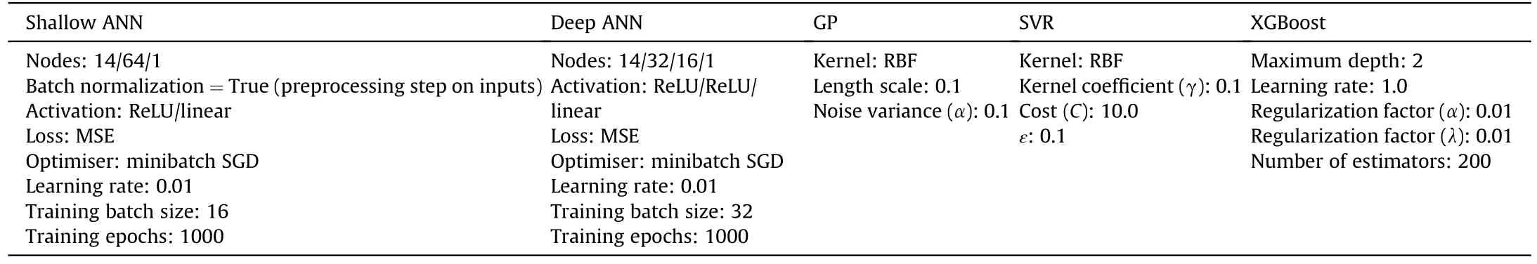
Table 2Details of the regression models and hyperparameters used for ballistic limit predictions following 5-fold cross-validation for hyperparameter selection.

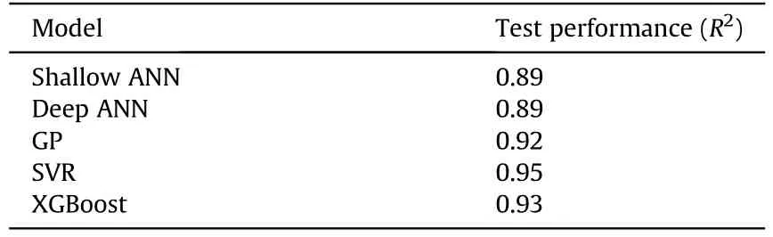
Table 3Performance of the different regression modelling approaches to predict V50 ballistic limit.

A summary of the models’ performance is provided in Table 3.The models are all shown to achieve relatively high predictive accuracy, withR2scores on the test dataset from 0.89 to 0.95.The shallow NN is found to outperform the deep ANN, suggesting that even with only 2 hidden layers the deep network is overparameterized.Some examples of the trained model outputs are provided in Fig.2 to give a qualitative indication of the model performance.From the examples provided we can observe that in the regions for which experimental data exists (i.e., the plot markers), within a thickness range of 22.9-54.8 mm for the AA2060-T68 and 41.2-78.4 mm for the ARMOX370, the models generally predict similar results.The GP,ANN,and SVR models are all shown to interpolate smoothly within these ranges, whereas tree-based methods like XGBoost model will not be smooth.Although such methods are typically hard to beat for tabulated datasets (particularly small datasets), see e.g.Ref.[25], their discontinuous outputs are likely unsuitable for use with physical systems.Beyond the limits of the training data, i.e., outside the thickness range of 22.9-54.8 mm for the AA2060-T68 and 41.2-78.4 mm for the ARMOX370,there is a substantial divergence between the predictions of the different models, indicating the inability of all these models to extrapolate to conditions outside those contained in the training dataset.The differing predictions of the various models outside the training data regime can be attributed to their respective formulations and hyperparameters.It can be noted in Fig.2 that the dependence of V50on thickness is linear over the range of experimental data.This suggests that the dominant penetration/perforation mechanism does not substantially change over the range of included velocities and target geometries.More generally, however, the wide range of target materials (and thus physical and mechanical properties), target thicknesses,projectile types,and impact conditions are expected to encompass a wide range of failure mechanisms.Indeed,this is a key benefit of the ML-based model - it is ’generally’ applicable across the range of input variables and failure mechanisms included in the training database, unlike most semi-analytical/empirical approaches which are often mechanism-specific or validated for only a very narrow range of variables (e.g., projectile types, target materials, impact conditions, etc).

Guidelines for reporting of results: model performance should be reported in terms of the evaluation metric defined in the methodology, applied to the test dataset.Performance on the training dataset can be reported in combination with the test data performance,but can only be used to identify e.g., overfitting (when the training performance is significantly higher than the test performance).If overfitting occurs,the performance of the trained model will be poor when it is being applied to predict the result for new data.For physical systems it is useful to present quantitative metrics such as R2 on the test data, together with qualitative outputs, e.g., the ballistic limit curves shown in Fig.2.

Fig.2.Comparing the regression model outputs for two representative projectile-target pairs.Experimental data points are indicated by the circular markers.The shaded region indicates the GP uncertainty.

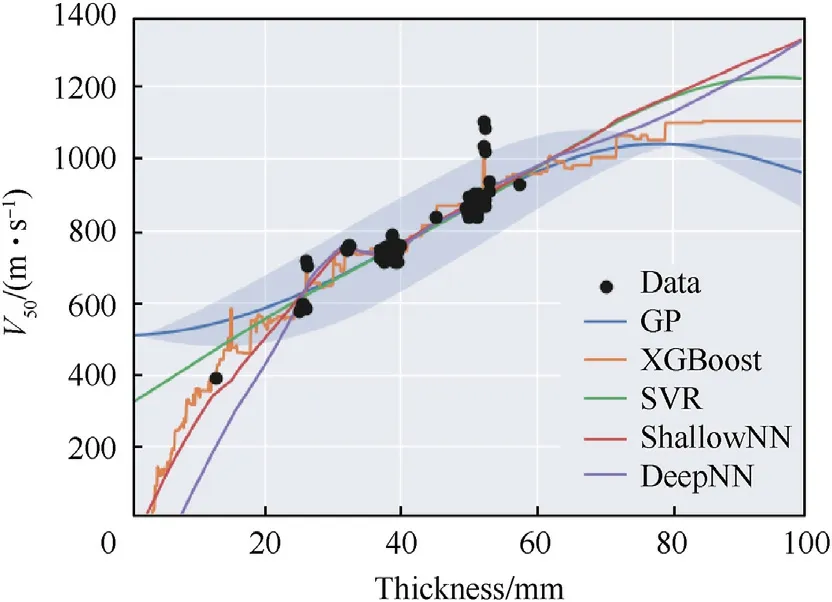
Fig.3.Comparing the regression model outputs against a very noisy subset of the experimental data - 7.62 mm APM2 projectiles at normal incidence.The shaded region indicates the GP uncertainty.Note that this is a 2D representation of a 13-dimensional GP.

2.4.Implications of noisy data

Terminal ballistic experiments are subject to scatter due to,amongst other factors,variations in plate thickness and mechanical properties (locally and differing across manufacturers and melts),projectile rotation/yaw,etc.For this study we retain all data in our database unless we have evidence to exclude it,e.g.,we can identify a typo in the original test records,etc.Such’noisy’data is handled differently by the approaches introduced in subsection 2.2.Most regression models,including ANN,SVR,and XGBoost,handle noise through regularization-a technique which effectively penalises a model as it becomes more complex.There are two main forms of regularization:Lasso(L1) and Ridge(L2).We useL2 regularization for our ANN and SVR models and bothL1 andL2 regularization in the XGBoost models.

Of the techniques we consider in this investigation,GPs have the most robust handling of noisy data.The statistical nature of the Gaussian process allows it to directly account for noisy observations by assuming that any measurement,y, is corrupted by some random noisey=f（x）+εnwhere εn～N （0，σn） for some predefined noise level σn.In subsubsection 2.2.3 we stated that the GP standard deviation will be near-zero at a sampled/experimental measurement.For a noisy system, "near-zero" should be replaced with the magnitude of noise present the experimental measurements.

In Fig.3 we compare the respective fits of the regression models on a very noisy dataset,7.62 mm APM2 projectiles against AA6061-T651 at 0°.For targets 50.8 ± 1.0 mm thick the experimental variation in the recordedV50is extreme: 837-1102 m/s.We can observe that the GP,SVR,and shallow NN provide a similar fit to the thickness range in which data is available, regressing through the centre of the data cluster at a thickness of 50.8 mm.The deep NN and XGBoost are observed to overfit the data.The uncertainty of the GP is shown as a shaded region, demonstrating the variance magnitude in instances of noisy data.

The effect of the noisy data on the assessed model performance is such thatR2values = 1 will never be achievable.

2.5.Dimensionality reduction

We have a 14-dimensional input space and approximately 700 data points in the training dataset, which is quite sparse when we consider that the data is also highly clustered (e.g., ＞20% of the dataset is for 7.62 mm APM2 projectiles against AA6061-T651 at normal incidence,etc.).Here we utilise feature importance ranking(FIR) and feature correlation to reduce the dimensionality of the input space.FIR is a means of measuring and ranking the contribution of individual inputs to the model outputs.It is most readily performed by tree-based methods such as XGBoost.Our feature space contains some obviously correlated variables, for instance:target yield strength,hardness,and tensile strength.We can utilise FIR and a correlation assessment to remove variables that (a) are highly correlated to other input features, and thus their influence should be transferrable to those correlated features if removed,and(b) input features that have minimal influence on the model outputs, and thus can be removed without loss in performance.

The 14 input features are ranked for their influence on model output in Fig.4.Here we can observe that the most influential features are projectile calibre, target thickness, target density, and projectile mass, while the least influential features are Poisson’s ratio, target strain hardening exponent, and projectile density.Some of these are unexpected,e.g.,projectile density,etc.,however this is likely due to feature correlation (i.e., projectile density and calibre will correlate strongly with projectile mass, and thus it’s influence on the output can be diffused in FIR).In Fig.4 we also show the correlation between input features, noting that as expected some features are highly correlated (e.g., target density,modulus,hardness,UTS,and yield strength).We reduce the feature space based on a combination of the FIR ranking and expert choice(based on experience).The reduced feature space includes projectile calibre, density, and hardness, together with target thickness,density, hardness, and impact angle.Although yield strength is ranked higher than hardness in the FIR, hardness is our preferred strength feature as many of the experimental records report a measured hardness.

Fig.4.(a) Feature importance ranking (from XGBoost model), the input features removed for the reduced complexity model are de-emphasised; (b) Correlation (Pearson’s correlation coefficient) of the input features.Note that ‘PR’ is Poisson’s ratio and UTS is ultimate tensile strength.

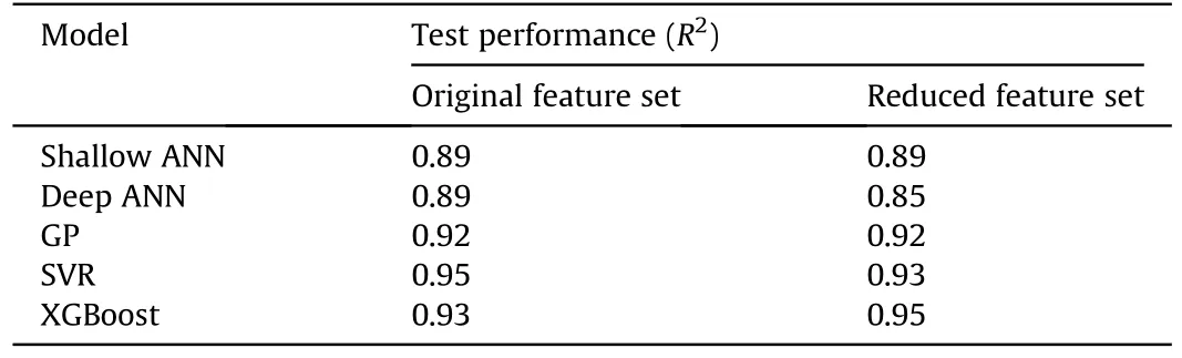
Table 4Comparing the performance of the different regression modelling approaches with reduced feature set to predict V50 ballistic limit.

It should be noted that the FIR shown in Fig.4 is determined for the entire dataset.For specific subsets of the data, i.e., a particular combination of projectile type and target material, a different ranking of the feature importance would be achieved.It should also be noted that the database is dominated by AP-type projectiles on aluminium alloy targets (see Fig.1).For this combination of projectile and target the dominant failure mechanism is ductile hole growth,a mechanism highly correlated to target strength.Thus,it is expected that target material yield strength ranks highly in the FIR.

We retrain the regression models, using the same approach as described in subsection 2.3, on the reduced input space (dimensionality reduced from 14 to 7)and report the results in Table 4.We can observe that the change in performance of most models is modest,with the XGBoost showing a modest improvement and the deep NN and SVR showing a modest decrease.We cannot conclude that the data reduction has any meaningful effect, positive or negative, on the model training.

Guidelines for model selection: There is a wide range of machine learning models suitable for use in regression problems, each with their own strengths and weaknesses.Model selection should be informed by the application,data volume (i.e., number of features and number of samples),problem complexity,etc.as well as with the end application in mind.For instance, tree-based methods such as XGBoost, although often amongst the best performing models for regression and classifications,particularly those with limited volumes of training data, are typically unsuitable for predicting the continuous behaviour of physical systems due to their nested if/then decision point architecture leading to a non-smooth output (see e.g., Fig.2).In general, shallow neural networks (i.e., one hidden layer)provide a good balance of flexibility and capability for most regression tasks in terminal ballistics.GP regression models are more computationally expensive but provide mathematically sound uncertainty predictions so are preferred for application in probabilistic assessments, e.g.,survivability/lethality calculations.

2.6.Physics-informed machine learning

Regression models have no actual understanding of the problem on which they have been applied, they merely identify patterns between the input and output features.Thus, application of such models should be limited to the range of input conditions encompassed by the training data.However,if we have knowledge of the underlying physics of the system that we are attempting to model,we can incorporate that knowledge while training the ML model.This is known asphysics-informedmachinelearning(PIML),see e.g.,Ref.[26].By utilising our prior knowledge of the physical system,PIML can both reduce the volume of training data typically required for machine learning models to achieve good performance and allow for the model to be used for conditions outside the training dataset (only if the physics-based model is valid for those new conditions).For terminal ballistics problems in which we (a) can expect to have limited data, and (b) can often need to interpolate between the experimental data points and extrapolate beyond them, PIML is particularly attractive.

2.6.1.Enforcedmonotonicity

One of the simplest PIML approaches is to enforce a monotonic relationship between an input variable and the system output, for example in ballistics we would typically assume a monotonic relationship between impact target thickness andV50ballistic limit(if all other variables are constant).For an ANN monotonic constraints can be implemented in a soft manner, in which the assumption can be violated but at a cost in the loss function (e.g.Ref.[27],etc.),or in a rigid manner,in which the architecture and/or learning process used to train the model are such that it is impossible to violate the constraint (e.g.Ref.[28], etc.).

We incorporate a point-wise loss (PWL) function [27] that incorporates monotonic knowledge into our shallow and deep neural networks by altering the learning process(i.e.,a soft enforcement).The typical MSE loss function we are using to train the neural networks is given by Eq.(1).To enforce monotonicity the loss function is modified:

where ∇·Mis divergence with respect to the monotonic feature set,x［M］.For enforcing monotonicity on thickness, i.e.,x［t］

and θ are the connection weights of the network.

Effectively, Eq.(3) states that if monotonicity of output feature,V50,with respect to the input feature thickness,t,is valid about thei-th experimental point,then the corresponding loss for that point is simply the MSE loss from Eq.(1).However, if the monotonicity constraint is violated,then the loss includes an additional term,Eq.(4),the magnitude of which is dependent on the magnitude of the violation.

We demonstrate the effect of the monotonicity constraint applied to the input featurethicknessin Fig.5 for the shallow and deep neural networks and report the performance metrics in Table 5.We can see in Table 5 that the monotonicity constraint has very little effect onR2for both the shallow and deep NNs,providing a modest improvement.For most target-projectile-angle groups we observe marginal difference between the model outputs, particularly in the regions with data.The 30 mm APDS plot shown in Fig.5 indicates a positive qualitative effect of the constraint, specifically preventing a negative slope of theV50curve with respect to thickness(i.e.,non-physical relationship).However,the monotonic constraint for the 30 mm APDS projectile also results in a degradation in quantitative predictive accuracy, specifically for the～50 mm thick target.

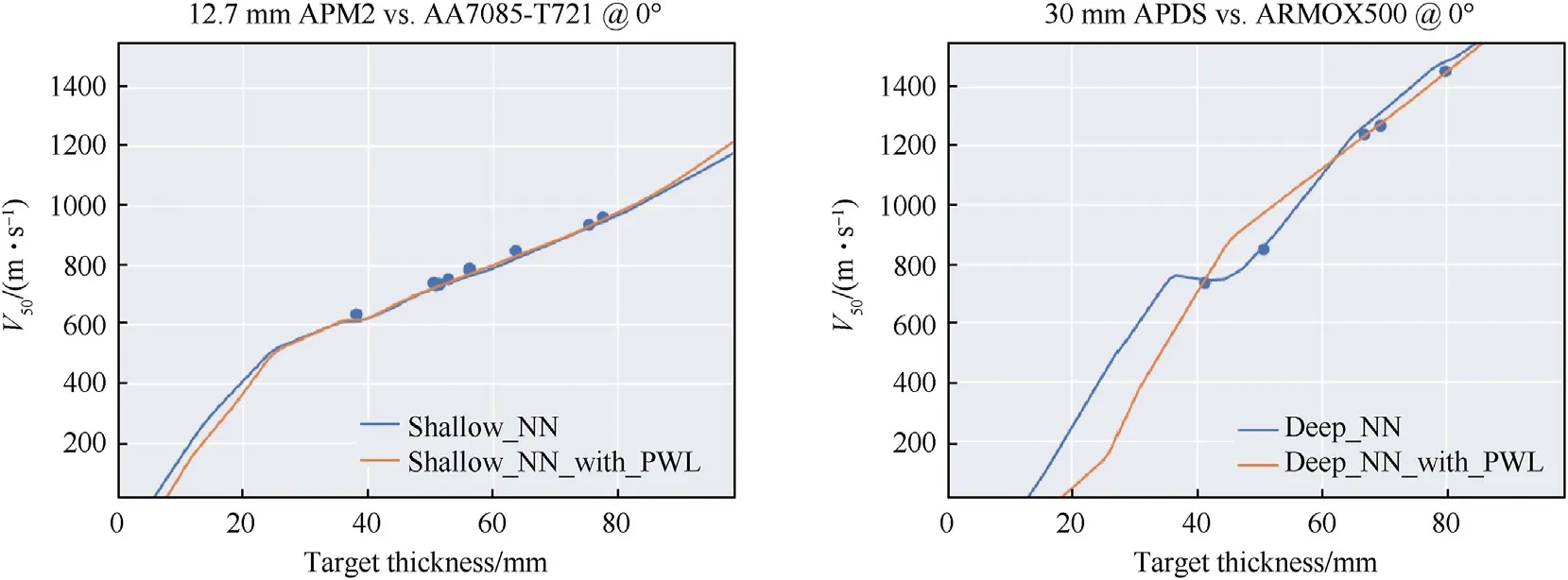
Fig.5.The effect of enforced monotonicity between input feature’thickness’and output feature’V50’,for shallow and deep neural networks on two representative projectile-targetobliquity combinations.

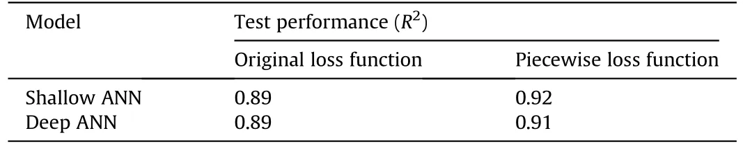
Table 5Performance metrics for the neural networks trained using the full input feature space(14 features)with the original loss function,Eq.(1),and the PWL function,Eq.(3), applied to enforce monotonicity between target thickness and V50.

2.6.2.Gaussianprocesswithnon-zeropriormean

The GP prior mean is usually set asm（x）=0 to simplify calculations.This approach was used in the preceding sections.However,if we have a physics-based equation that we know is approximately true, we can use utilise that information by incorporating it as a prior mean.Effectively this means that the Gaussian process will agree with the data in regions where we have it,but it will revert to the physics-based model in regions with no data.To incorporate this model, we use the property of expectations that E［f（x）-m（x）］=E［f（x）］-m（x） sincem（x） is a scalar function.This means we can train the computationally simpler zero prior mean Gaussian processg（x）=f（x）-m（x）and just addm（x）to the result.

Form（x）we need an equation that can prediction ballistic limit velocity,Vbl,which we use interchangeably withV50in this analysis,consistent with e.g.,Ref.[29].HereVblis a deterministic measure of ballistic limit velocity, comparable toV50without the additional statistical information (and thus alternative measures such asV10andV90cannot be determined fromVbl).In engineering practiseV50is typically greater thanVbl[30] due to its means of calculation,however, for this analysis that variation is treated as negligible.Although there exist many empirical and semi-analytical models for predicting the performance of monolithic metallic plates perforated by projectiles, none are general in the sense that they can be widely applied irrespective of projectile and target material,projectile type (e.g., rigid, deformable, nose-pointed, blunt, etc.),and impact condition (i.e., velocity and obliquity).Amongst the simplest ballistic conditions is that of a ductile plate perforated by a rigid penetrator through ductile hole growth,a condition for which the ballistic limit can be estimated via cavity expansion theory,

whereris the projectile radius,mpis the projectile mass,his the target thickness,Cis a constant referred to as the shape factor which defines the thickening at the edge of the expanded hole,and σ is the stress at the edge of the expanding hole.There are several formulations of Eq.(5)that vary primarily in their definition of theCσ product,including classical works by Taylor[31],Bethe[32],and Hill[33].More recently Forrestal and co-authors,e.g.Ref.[34],have developed a plane-strain formulation of a quasi-static radial stress while Masri and co-authors, e.g.Ref.[35], have developed a formulation based on the cavitation effective yield stress,

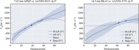
Fig.6.Comparing outputs of a Gaussian process regression model(“GP”),ductile hole formation based semi-analytical model(“Masri”)and physics-informed GP(“PI-GP”)that uses the Masri model as a prior mean with ballistic experimental data.The shaded region indicates the 95% confidence bound of the PI-GP.

wherehis the target thickness,Eis the Young’s modulus of the target material,Dis the calibre/diameter of the near-rigid projectile core, γp=4mp/πD2is the projectile areal density, andis the cavitation effective yield strength [24]:

where φ =2/（3Σy）,Σyis the yield strain,Yis the yield stress,β =1-2ν,ν is Poisson’s ratio,andnis the strain hardening exponent in a modified Ludwik power-hardening law,

The ductile hole formation scaling law,Eq.(6),referred to herein as theMasrimodel, has been demonstrated to provide very accurate predictions(within a few%typically)when applied to a range of aluminium alloys impacted by AP projectiles, see e.g., Ref.[36].Comparable performance models for ball- and fragment-type projectiles do not exist, see e.g., Ref.[37].Importantly, our implementation assumes that the model is only approximately true-in the absence of data the ML models will revert to the equation as a worst case,but in the presence of data that varies from the equation predictions,the models will fit the data.Thus,we will apply Eq.(6)for all projectiles, realising that the performance will vary significantly depending on projectile type.

In Fig.6 we plot the model outputs of the basic GP from subsection 2.2 and physics-informed GP (PI-GP) together with the semi-analytical model, Eq.(6), and experimental data.The examples are provided for conditions at which the Masri model can be validly applied(i.e.,ductile hole growth-dominated conditions),to demonstrate the effect of the model on the PI-GP output more clearly.We can observe in Fig.6 that in the presence of experimental data there is minimal difference between the GP and PI-GP,both provide an excellent fit to the experimental data.At velocities above and below the experimental data the GP begins to return to the standardised mean of the database while the PI-GP returns to the physics-based model prediction.This result highlights some preferrable characteristics of the PI-GP, compared to the basic GP,e.g., it proceeds to aV50→0 as thickness approaches 0, V50monotonically increases with thickness, etc.

A comparison between the performance of the various models,separated into projectile classes,is provided in Table 6.We separate the"AP"type projectile results into subclasses"Masri"and"Other",where the Masri sub-type contains those experimental conditions for which the model can be validly applied, specifically: those at normal incidence, those where quasi-rigid core penetration can reasonably be assumed - here we use only impacts against aluminium targets, and those in which the target plates are sufficiently thick that petalling or dishing are not the dominant failure modes(here we assume to beh/D＞0.5).In our database there are no targets in which the target thickness is sufficiently high that inertia needs to be considered.The PI-GP is found to achieveR2= 0.95, compared to 0.92 for the standard GP from subsection 2.2.The physics-based model has anR2of 0.64 when applied to the test dataset, which is unsurprising given that the model is only expected to be accurate for conditions which result in perforation via ductile hole growth.For those experiments on which the Masri model can validly be applied,according to its derivation,the model has anR2score of 0.87,slightly lower than the results from Ref.[36](R2= 0.95 when applied to a different database).

Given that the Masri model is applied beyond its valid range the overall predictive performance is poor.So, the question becomes how can a poorly performing model improve the prediction of the GP? As discussed in subsubsection 2.2.3, a GP will return to the prior mean in the absence of observational data.Typically, this would be the Gaussian mean of the scaledV50values in the training dataset as we adopt a scaled prior mean of zero.Inclusion of the physics-based model, even if it is only approximately accurate,provides additional knowledge to the GP that results in improved performance.The obvious limitation of this approach is when the PI-GP model is used to the predict the performance of projectile/target/impact condition combinations that are (1) not valid applications of the Masri model, e.g., fragment-simulating projectiles,and (2) are extrapolations beyond the training data regime for projectiles.In this case the prediction will correspond to that of the Masri model(i.e.,it will be a poor prediction as it is being applied to a non-valid condition for the model).

We have developed ’general’ ML models by training them on a database containing a wide range of projectile types, target materials,geometries,impact conditions etc.One of our motivations for this approach is the absence of more publicly availableV50data.Given more data,an alternate approach would be to build a series of less general models, e.g., projectile specific models, material specific models, mechanistic specific models, etc.These models could potentially incorporate physics-based models such as the Masri model without violating their validity bounds,i.e.,if the ML-model was specific and trained only on experiments with AP projectiles impacting aluminium targets at normal incidence for geometries and velocities at which ductile hole growth is the dominant mechanism.For relatively simple projectile-material-condition-mechanism schemes, such as ductile hole growth by rigid penetrators, there would be little use for such models as the existing analytical approaches are fast, accurate, and provide more insight into the relevant inputs than a ML-model.For more complex schemes,e.g.,fragment simulating projectiles against steel targets,for which existing models have poorer performance (see e.g.Ref.[37],etc.)such models may be more attractive.However,given the limited ballistic data available in the public domain, such an approach is not feasible at this time.

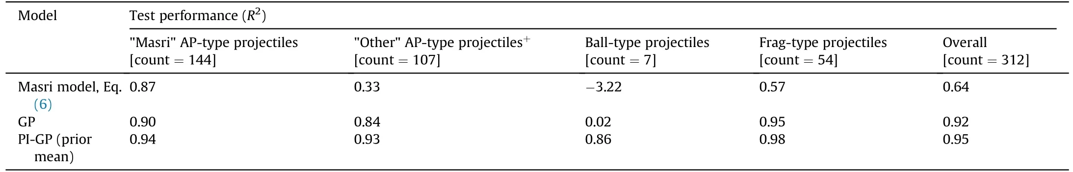
Table 6Performance metrics for the physics-informed GP model incorporating the ductile hole formation scaling law,Eq.(6),as a prior mean,compared with the standard GP applied to the test dataset.

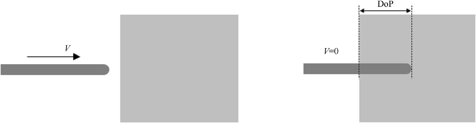
Fig.7.Impact of a long rod projectile at initial velocity V into a semi-infinite target block.The depth of penetration, DoP, is measured once the projectile ceases to penetrate.

3.Predicting depth of penetration

In Ref.[4] ballistic data is collated from many references for metallic projectiles penetrating into semi-infinite metallic target.A schematic of the problem is provided in Fig.7.

The database in Ref.[4] includes a wide range of projectile materials (e.g., steel, tungsten, aluminium, magnesium, gold,tantalum, etc.), target materials (e.g., steels, aluminium alloys, Pyrex, magnesium, lead, etc.), projectile geometries (L/D: 0.79-380)and impact conditions (V: 240-7500 m/s, θ: 0°-70°).A statistical analysis of the database is provided in Ref.[3].

Here we repeat some of the steps performed in section 2 to demonstrate the applicability of the methodology to another common terminal ballistics problem.In Ref.[3]an ANN was trained on the dataset from Ref.[4], thus we also provide a comparison with the methodology and results from Ref.[3].

3.1.Regression modelling

We utilise the same four regression modelling approaches as detailed in subsection 2.2, namely: XGBoost, ANN (shallow only),GP, and SVR.We utilise the same hyperparameter tuning and training methodology as previously defined.Details of the modelsare provided in Table 7.For the shallow ANN we reproduce the network architecture and loss function used in Ref.[3].

Table 7Details of the regression models used for depth of penetration predictions.

We first consider regression of the following input features:projectile velocity(V),projectile aspect ratio(length/diameter,L/D),projectile density (ρp), projectile hardness (BHNp), target density(ρt),and target hardness(BHNt)[input feature vector length=6],to the output feature penetration/projectile length (P/L).The performance of the four models on the test dataset is provided in Table 8.Additionally,trained models are applied to generate velocity vs.P/Lcurves in Fig.8 for long(length/diameter,L/D=10)and short steel rods(L/D=1)impacting on a steel target[6].The curves generated by the GP,ANN,and SVR models are relatively similar in Fig.8,with the ANN qualitatively appearing the worst due to the apparent overfitting.The GP, in addition to providing good qualitative and quantitative outputs also provides mathematically sound uncertainty predictions, shown as the shaded region in Fig.8.The XGBoost model,although scoring the highest on the test dataset,is likely unsuitable for use due to its discontinuous nature.

3.2.Dimensionality reduction

To try and improve model performance Rietkirt et al.[3]utilised the BuckinghamPitheorem[5]to generate non-dimensional input features.The π-groups (defined below) can be considered as engineered input features, which are commonly used in machine learning to improve the relevance of inputs and reduce the dimensionality of the input feature space.

The regression models presented in subsection 3.1 were trained on the engineered input features from Eq.(9) (as per [3]) and the results are provided in Table 9,compared to the models trained on the original features.We can observe that the ANN and GP experienced modest improvements in performance when trained on the engineered features,but the SVR and XGBoost models experience a modest performance decrease.With the exception of the SVR model, we cannot conclude therefore that the dimensionality reduction using engineered features has any significant effect on the model performance, contradicting the conclusion in Ref.[3]who stated that the engineered features resulted in an improvement in model performance.

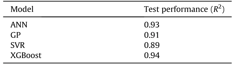
Table 8Comparing the performance of the different regression approaches for predicting depth of penetration.

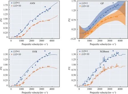
Fig.8.Predictions of the four regression models applied to two series’ of steel penetrators (230 BHN) impacting upon steel targets (295 BHN) compared to experimental measurements.

A comparison between outputs of models trained on the ’original’ (or ’raw’) input features compared with the ’engineered’ features is given in Fig.9 for two representative cases:the ANN applied to theL/D=10 data and the GP applied to theL/D=1 data.We can see that the performance of the GP trained on the raw features is clearly superior to that of the GP trained on the engineered features, particularly in the low velocity range.For the ANN there is less of a difference,however the raw model appears to fit the data marginally better.The plots show only one configuration on which the model is trained, and as noted in Table 9 we would expect the ANN trained on the engineered features to outperform that trained on the raw features over the entire test data set.

3.3.Physics-informed machine learning

3.3.1.Gaussianprocesswithnon-zeropriormean

As per the methodology introduced in subsubsection 2.6.2,if we have physics-based equations that we know are approximatelytrue, they can be used to complement our experimental data that we know is absolutely true (to within experimental scatter).Here we employ the modified hydrodynamics theory of Tate [38] and Alekseevskii [39] to generate a closed-form prediction of penetration to underpin our PIML approach.The Alekseevskii-Tate model is strictly applicable to rod-type penetrators only and has known limitations in predicting residual penetration when the projectile strength,Yp, is greater than the target resistance,Rt, i.e.,Yp＞Rt.Definition of the projectile and target strength terms is also problematic.However, as we assume that the model is only approximately true we consider it reasonable to apply the model to the entire dataset.Penetration depth into a semi-infinite target,P∞, is calculated by integrating the interface velocity (i.e., the velocity at the interface of the projectile and target materials),u, over the duration of the penetration event,t,

Table 9Evaluating the effect of engineered input features on regression model performance for the depth-of-penetration dataset.

where the interface velocity is determined from a modification of Bernoulli’s theorem, given in Tate’s notation by:

For calculating the projectile strength,Yp,and target resistance,Rt, terms we use the approach from Ref.[40]:

Fig.9.Comparing the fit of models trained on original input features("raw features")and Buckingham π-groups("engineered features")with combined training and test data for the ANN, left, and GP, right.

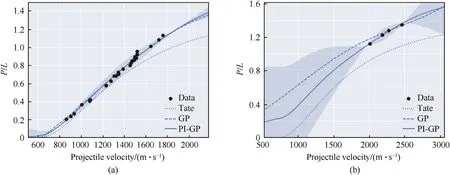
Fig.10.Comparing outputs of the GP model trained on original input features("GP"),the physics-based model of Alekseevskii and Tate("Tate")and the physics-informed GP("PIGP")model that incorporates the physics-based model as a prior mean with experimental data for L/D=10 WHA projectiles into two semi-infinite steel targets:264 BHN(a)from and 390 BHN steel (b) from Ref.[43].The shaded region indicates the 95% confidence interval of the PI-GP model.

where σy=3.92×BHN(MPa) [41].

Tate defines special conditions related to the projectile strength and target resistance,an in-depth derivation and review of which is provided in Ref.[42].

As per subsubsection 2.6.2 we incorporate the Alekseevskii-Tate prediction as a prior mean to the GP.In Fig.10 we plot the Alekseevskii-Tate model together with the basic GP (from subsection 3.1) and the physics-informed GP ("PI-GP") that uses the physics-based model as a prior mean, together with the experimental data.For Fig.10(a)there is little difference between the GP and PI-GP as we’re plotting in a regime relatively well populated by experimental data.The Tate model, for this projectile-target combination, is shown to provide accurate predictions at lower velocities, increasingly underpredicting the penetration depth with increased velocity.In Fig.10(b) we show a projectile-target combination with less experimental data,resulting in a larger difference between the GP and PI-GP.The experimental data is at velocities above 2000 m/s, where the Tate model is shown to again underpredict penetration depth.As a result,the PI-GP is shown to predict lower penetration across almost the entire velocity range plotted,compared with the GP.About the experimental data the difference between the GP and PI-GP is minimal.The performance of the GP and PI-GP is compared in Table 10.We separate the data into"Tatevalid" and "other" based on projectileL/D, with "Tate-valid" for experiments with projectileL/D≥9.8 and "other" for projectileL/D＜9.8.We can observe a substantial reduction in performance for the Tate model when applied to the "other" experimental data samples,yet the GP and PI-GP continue to perform well across both highL/Dand lowL/Ddatasets.

4.Conclusions

Machine learning (ML) is emerging as a useful tool in the analysis and prediction of terminal ballistic events due to its ability to identify patterns and trends in high-dimensional data that may be imperceivable to human experts.We have applied several ML regression modelling approaches for two common terminalballistics problems: (1) predicting the ballistic limit of monolithic metallic targets impacted by different classes of small-and medium-calibre projectiles, and (2) predicting the penetration depth of projectiles impacting target plates of semi-infinite thickness.The regression models,including extreme gradient boosting(XGBoost),artificial neural network (ANN), support vector regression (SVR),and Gaussian process regression (GP) typically exhibit comparable performance-all achieving excellent agreement with the training data.

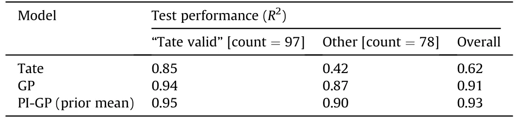
Table 10Performance metrics for Gaussian process (GP) trained using the original input feature space (6 features) and physics-informed GP (PI-GP), using the Alekseevski-Tate model, Eq.(10) as a prior mean.

ML-based regression models are not normally suitable for extrapolation to conditions beyond that encompassed by the training data and can be inaccurate when interpolating across sparse data regimes within the domain of the training data.This is evidenced by the divergence of the ML-regression models at impact velocities above and below the limits of our training data.Such divergence makes these models unsuitable for application in survivability and lethality analyses.To overcome this limitation, we present techniques for incorporating expert knowledge in the MLregression models,including enforced monotonicity between input features such as target thickness and system output (e.g., ballistic limit),and via physics-based models-specifically cylindrical cavity expansion and modified hydrodynamics theory.These physicsbased models are utilised as a prior mean of a Gaussian process,resulting in a model that,in the presence of experimental data will fit that data, but otherwise will revert to the physics-based model prediction.This is a powerful approach that enables the state-ofthe-art analytical or empirical approach to be maintained, whilst improving the model’s agreement with experimental data.

Declaration of competing interest

The authors declare that they have no known competing financial interests or personal relationships that could have appeared to influence the work reported in this paper.