Numerical Assessment of a Class of High Order Stokes Spectrum Solver

Etienne Ahusborde,Mejdi Azaïezand Ralf Gruber

&Pays Adour,F d ration IPRA,UMR5142,64000,Pau,France.

2Bordeaux INP,I2M(UMR CNRS 5295),33607 Pessac,France.

3Chemin du Daillard 11,1071 Chexbres/VD,Switzerland.

1 Introduction

The 2D Stokes eigenvalue problem on a square domain is considered in this paper as model example with a conservation law of the type ∇·u=0.With this test example it is possible to discuss the various numerical problems that appear when flux conservation has to be satisfied in the incompressible Navier-Stokes.If these constraint condition cannot be satisfied precisely,so-called spectral pollution[9]appears and the numerical approach does not stably converge to the physical solution.The reason is that due to regularity constraints imposed by standard numerical approximation methods,the energy cannot reach the minimum required by the physics.In fact,current numerical methods satisfy the boundary conditions strongly,the operator equations and the constraints only weakly.

In Section 2,we propose a non-exhaustive list of methods to deal with the 2D Stokes eigenvalue problem.Specifically,if the constraint∇·u=0 is satisfied by au=∇×ψansatz,the number of degrees of freedom remains the same as in the unconstrained Laplacian problem.As a consequence,besides the Stokes modes,one finds a whole spectrum of additional unphysical modes,corresponding to those of the heat equation.Thus,the initial physical problem has fundamentally been changed.This approach has been applied to compute the full Stokes spectrum[1]by the first time.Due to the choice of a unit square domain,the authors were able to separate the Stokes modes from those belonging to the heat equation.An other strategy consists in applying a penalty method to solve the Stokes problem.In this case,the number of degrees of freedom still remains the same as those in the unconstrained Laplacian problem.

In Section 3,we focus on the two formulations considering only the velocity as variable:the penalty method and the divergence-free Galerkin approach.In the framework of spectral element approximation schemes,a stable spectral element is proposed for each method.For the penalty method,a COOL approach[2,3]is made and the unphysical modes can be pushed towardsλ=0.For the divergence-free Galerkin approach,two strategies christened “explicit” and “implicit” are detailed.The explicit strategy consists in using the properties of the kernel of the grad(div)operator to construct a divergence free basis.Such a basis has the right number of degrees of freedom,thus delivering the exact number of Stokes eigenfunctions with high precision.The implicit strategy is a direct algebraic elimination process of the ∇·u=0 constraint.This leads to a sparse matrix elimination process,described in detail in[2].It delivers the right number of highly precise Stokes modes.

Finally,in Section 4,some numerical experiments are performed to prove the efficiency of the proposed methods and a comparison between the different approaches is given.

2 The Stokes eigenvalue problem:continuous version

Let Ω ⊂IRd,d=2,3,be a Lipschitz domain,the generic point of Ω is denotedx.The symbolL2(Ω)stands for the usual Lebesgue space andH1(Ω),the Sobolev space that involves all the functions that are,together with their gradient,inL2(Ω).C(Ω)denotes the space of continuous functions defined in Ω.

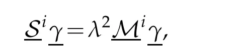
The continuous Stokes eigenvalue problem reads:Find a vector u and λ2∈IR+suchthatwhereIR+denotes the set of positive real numbers,including zero.For the sake of simplicity we assume here that Ω is the reference domain(−1,+1)2.

Problem(2.1)is often solved using different strategies that we briefly recall here after.

Velocity-Pressure formulation

Its weak formulation writes:Find u∈and λ2∈IR+such that

Stream function approachWe introduce a stream functionψ∈H2(Ω)d[1].Problem(2.1)can be reformulated as:

However,in this paper we prefer to focus on methods involving onlyuas unknown.The first one is calledPenalty method.

Penalty method This method consists in taking into account the divergence free constraint by adding a term of penalty to control the level of divergence when solving the eigenvalue problem.

The penalty formulation,called also regularization method(see[8]),reads:Find u∈((Ω))2and λ2∈IR+such that

Its variational formulation writes:Find u∈((Ω))2and λ2∈IR+such that

In practice,the infinite dimensional problem(2.6)is replaced by a finite dimensional one using a stable spectral element taking into account the constraint by an adequate choice ofα(see[3]).

Divergence-free Galerkin approachThe second method is called”divergence-free Galerkin approach”and starts from the fact that the system(2.6)can reduce to:Find u∈Xand

λ2∈IR+such that

where X is in the space defined by

Again the infinite dimensional problem(2.7)is replaced by a finite dimensional one using a stable spectral element that will be developed later in this paper.

3 The Stokes eigenvalue problem:discrete version

We firstly introduce some notations and reminders.Let ΣGLL={(ξi,ρi);0≤i≤p}and ΣGL={(ζi,ωi);1≤i≤p}respectively denote the sets of Gauss-Lobatto-Legendre and Gauss-Legendre quadrature nodes and weights associated to polynomials of degreep.These quantities are such that on Λ :=]−1,+1[

whereIPp(Λ)denotes the space of polynomials with degree≤p.We recall that the nodesξi(0≤i≤p)are solution to(1−x2)(x)=0 whereLpdenotes the Legendre polynomial of degreep,whereasζi(1≤i≤p)are solution toLp(x)=0(see[4]).

The canonical polynomial interpolation basishi(x)∈IPp(Λ)built on ΣGLLis given by the relationships:

with the elementary cardinality property

where δijis Kronecker’s delta symbol.

We also introduce a new family of polynomials functions gi(x)associated to the canonical basis(3.3)through the relationships:

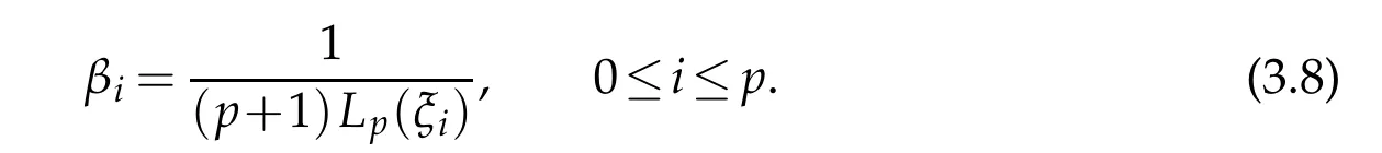
where the constants βiare such that all gi(x)∈IPp−1(]−1,+1[)[2,3].The functions gi(x)have the following properties:

1.Their moments up to order(p−1)are equal to those of their corresponding element in the Gauss-Lobatto-Legendre canonical basis,i.e.:For 0≤i≤p,

The difference(gi(x)−hi(x))being proportional to Lp(x)is orthogonal to all polynomials of degree less or equal to(p−1).

2.Interpolation of their corresponding element in the canonical basis at the Gauss-Legendre nodes,i.e.:For 0≤i≤p,

3.The constants βican be obtained through a series expansion of(3.3)and one gets:

In[3]one can read more informations concerning these polynomial functions.

3.1 Penalty method:SEM approximation

The discrete version of problem(2.6)writes:Find up∈Ypand λ2∈IR+such that

where:

Here(·,···)pis discrete scalar product based on Gauss Lobatto quadrature formula.Ypis the space of polynomial functions of degree lower or equal topvanishing on∂Ω.It is assumed to ensure a stable approximation for grad(div)operator to avoid the phenomenon of spurious pollution[3].Sinceupis equal to zero on the boundary,the solutionup∈Ypis approximated byaccording to the functional dependence and the regularity required(r=xory).

The superscript(1)is used to represent quantities derived in directionxwhile superscript(2)is used to represent quantities derived in directiony.The coefficients in the previous three expansions are the same thanks to(3.7).

Replacingupby the previous development in(3.9),the penalty discrete form writes

3.2 Divergence-free Galerkin approach

The keystone of the divergence-free Galerkin approach is the construction of a discrete versionXpof the divergence free space X defined in equation(2.8).

According to[2,5],we need the divergence to be a polynomial of degree less or equal top−1.Consequently,we want to build a space:

Expandingupaccording to(3.12b)and(3.12c)its divergence is a polynomials of degreep−1.Consequently,if the divergence is orthogonal to all polynomial ofIPp−1(Ω),it is necessarily equal to 0.This point gives a new characterization for Xp:

We want to build a basis of Xp.The first step consists in determining the size of this space.

wherep2is the number of necessary and sufficient equations to ensure ∇·up≡0.∇·up∈IPp−1(Ω)thereforep2≤p2.

There are 2 dependent equations in 2D(see[6]for details)since:

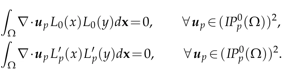
PolynomialsL0(x)L0(y)andare spurious modes and reduce the number of independent equations fromp2top2−2.Consequently,we requirep2=p2−2 test functionsqto ensure RΩ∇·upqdx=0.

After the computation of the size of Xp(denotedp1=(p−2)2in the sequel),we propose two strategies to compute a divergence-free basis.

3.2.1 Divergence-free Galerkin explicit approach

We consider the following eigenvalue problem:

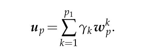
The kernel of the grad(div)operator includes all the modesassociated toλ2=0 and∇=0.It constitutes a basis for the subspace Xp.Its size is(p−2)2and thenup∈Xpcan be decomposed according to the following form:

Replacingupby the previous development in(2.7),the discrete variational formulation writes:Find up∈Xpand λ2∈IR+∗such that

This can be written:

The stiff matrix Seand mass matrix Meare symmetric and positive definite and are defined by:

for(1≤i,k≤(p−2)2).

3.2.2 Divergence-free Galerkin implicit approach

As highlighted before,the main difficulty of the problem(2.1)consists in satisfying the incompressibility constraint∇·u=0.Classical approaches usually satisfy operator equations strongly with as many equations as degrees of freedom for the velocity while incompressibility constraint is only satisfied weakly with fewer equations than degrees of freedom for the divergence.Contrary to the classical approaches,our objective is to favor the incompressibility constraint in comparison with the other equations.Our strategy,firstly introduced in[2],consists in sharing the degrees of freedom ofuin a relevant way to satisfy:

•The incompressibility constraint in strong sense.

•The other equations in weak sense.

Let upbe in Xp.The divergence of upis orthogonal to p2−2 polynomials of degree p−1.It is equivalent to saying that the divergence of up∈Xpnullifies in p2−2 Gauss points.The algebraic divergence equation writes Dup=0(see Figure(1)).

Figure 1:Algebraic system.

Figure 2:Decomposition of D.

D is a rectangular matrix with p2=p2−2 rows and 2(p−1)2columns.

Then,one splits D into D1⊕D2and upinto u1p⊕u2p(see Figure(2)).

Since,the p2−2 lines of D are independent,there is at least one choice of matrix D2invertible.Equation Dup=0 becomes:

For instance,u1contains the p1first values of upand consequently u2pcontains the p2remaining values.Figure 3 displays the sizes of the matrices D2and D1.

Since D2is invertible,the system leads to a relation between u1pand u2p:

Eq.(3.15)is crucial since it means that if we have any part u1pof up,we can build the complementary u2psuch that divergence of upequals 0.This argument allows us to build a basis of Xp.

Figure 3:Algebraic system=0.

We considervp∈((Ω))2.Our strategy consists in combining implicitly:

• A reduction fromvptov1p,

• An extension fromv1ptowp=(v1p,v2p)such that∇·wp=0 ensured by the multiplication ofv1pby the matrix

The matrixMis a two blocks matrix.The first block is a matrix of orderp1equal to identity.The second block containsp2rows andp1columns.It ensures the passage fromv1ptov2p.

• For eachvp∈((Ω))2,one associates a vectorwpof Xp.

By consequent,our strategy for the construction of a basis of Xpconsists in:

• Choosingp1=(p−2)2vectors()k=1,...,p1of the basis of((Ω))2(for instance,the(p−2)2first vectors),

• For each one of thesep1vectors,we consider itsp1-size reduced part denoted,

• We carry out the divergence-free extension

Thefamily is a basis of Xpand everyup∈Xpcan be decomposed according to the following form:

Replacingupby the previous development,the discrete variational formulation writes:Find up∈Xpand λ2∈IR+∗such that

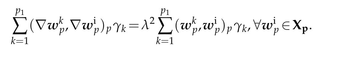
Table 1:Maximum and minimum of the L2(Ω)-norm of the divergence of all the Stokes eigen modes as a function of p.

This can be written:

with for(1≤i,k≤p1),

andrefer respectively to the Laplace operator and mass matrices expressed on the basiswp.

Finally,this system is equivalent to:

whereAandBrefer respectively to the classical Laplacian and mass matrices.

4 Numerical results

This section discusses some numerical results.We will apply each of the three approaches to compute the Stokes eigenvalues and associated eigenfunctions.

Penalty approachFigure 4 displays the convergence for the lowest eigenvalue of problem(2.5)for several values ofα.

One can see that the choice ofαleads to slightly different convergence behaviors.For double precision arithmetic,α=107appears to give the best convergence results.With an increasing polynomial degree to represent the eigenfunction,the eigenvalue converges exponentially as expected forp≤9.Increasingpfurther does not improve the accuracy of the eigenvalue,with the precision limited to 10−6.Table 1 shows the limit in precision for the incompressibility condition forα=107as a function ofp.

The eigenvalue problem(3.9)gives 2(p−1)2eigenvalues and associated eigenvectors corresponding to the degrees of freedom inYp.Among these eigenvalues,there are the Stokes eigenvalues and the non-zero eigenvalues of the grad(div)operator multiplied byα.The number of Stokes eigenvalues NScorresponds to the size of the kernel of the discretized grad(div)operator,i.e.to the number of zero eigenvalues.As said in Section(3.2.1),it can be proved that this number is equal to(p−2)2.Consequently,the resolution of the problem(3.9)leads toNS=(p−2)2Stokes eigenmodes.Thep2−2 remaining eigenmodes are those of the class of non-zero eigenvalues of the grad(div)operator multiplied byα.

Figure 4:Convergence plots obtained using the penalty method for the first Stokes mode(λ2=13.086172791)as a function of the polynomial order p for several values of α.

Figure 5 illustrates the convergence of the differenceǫbetween the four lowest Stokes eigenvalues as a function ofpcomputed by our method with those produced in[1]forα=107on a semi-logarithmic scale.The error is exponentially decreasing as expected forp≤11 and then stagnates.

Divergence-free Galerkin explicit approachFigure 6 illustrates the convergence of the differenceǫbetween the four lowest Stokes eigenvalues as a function ofpcomputed by the divergence-free Galerkin explicit approach with those produced in[1]on a semilogarithmic scale.The error is exponentially decreasing as expected.

Divergence-free Galerkin implicit approachTo validate our divergence-free Galerkin implicit approach,we have computed the Stokes eigenvalues and compared with those obtained in[1].Figure 7 shows the convergence for the four lowest eigenvalues as a function ofpon a semi-logarithmic scale.The calculation of the eigenvalues converges exponentially as expected.

It has been shown theoretically that the eigenmodes have a global structure with an infinite series of Moffat corner vortices[7]of increasingly smaller amplitude.The right part of the Figure 8 represents theupxcomponent of the thirteenth eigenmode.The amplitude is 0.852.In the center of the figure,we can see the first Moffat vortex in the left upper corner of the geometry with an amplitude of 1×10−3.At last,in the left side of the figure,the second Moffat vortex has an amplitude of 2×10−6.These results are in accordance with the theoretical ones.

Figure 5:Convergence plots obtained using the penalty method for the four lowest divergence-free modes as a function of p.Again,α=107.

Figure 6:Convergence plots obtained using the divergence-free Galerkin explicit approach method for the four lowest divergence-free modes as a function of p.

Figure 7:Relative error ǫ for the for the four lowest Stokes eigenvalues as a function of p on a semi-logarithmic scale with the divergence-free Galerkin implicit approach.

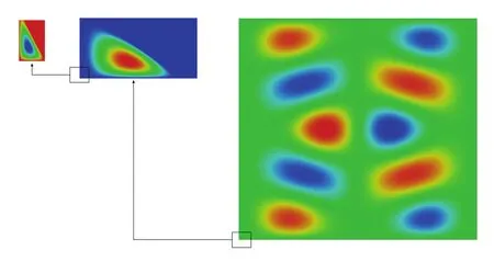
Figure 8:upxcomponent of 13thStokes eigenvector:Moffatt vortices in the corners.

Comparison between the different approachesThe three strategies described in this paper give the expected number of Stokes eigenvalues with a high precision.Nonetheless,Figure 5 compared with Figure 6 and Figure 7 indicates that the penalty approach is less accurate that the two other ones.Moreover,the divergence of the eigenvectors computed by the penalty approach is not identically null and its level can depend on the tricky choice of the values ofα.On the contrary,the divergence-free Galerkin approaches computed eigenvectors that are perfectly divergence-free.As drawback of the explicit version,we can mention that an initial computation of the kernel of the discretized grad(div)operator has to be performed leading to the resolution of two eigenvalue prob-lems.Consequently,due to the reasons mentioned above,in our opinion,among the three strategies studied in this paper,the best one is the divergence-free Galerkin implicit approach.

[1]E.Leriche and G.Labrosse,Stokes eigenmodes in a square domain and the stream function velocity correlation,Journal of Computational Physics,200(2004),489-511.

[2]E.Ahusborde,R.Gruber,M.Azaïez and M.L.Sawley,Physics-conforming constraints oriented numerical method,Physical Review E,75(2007),056704.

[3]E.Ahusborde,M.Azaïez and R.Gruber,Constraint oriented spectral element method,Lecture Notes in Computational Science and Engineering,76(2011),93-100.

[4]M.O.Deville,P.F.Fischer,and E.H.Mund,High-order methods for incompressible fluid flow,Cambridge University Press,Cambridge,2002.

[5]E.Ahusborde,High order method for the-grad(div)operator and applications,PhD thesis,University of Bordeaux,2007.

[6]C.Bernardi and Y.Maday,Spectral methods in handbook of numerical analysis,P.G.Ciarlet and J.L.Lions,North-Holland,1997.

[7]H.K.Moffatt,Viscous and resistive eddies near a sharp corner,Journal of Fluid Mechanics,18(1964),1-18.

[8]V.Girault and P.Raviart,Finite element methods for Navier-Stokes equations,Series in Computational Mathematics,Springer-Verlag,Berlin,1986.

[9]R.Gruber and J.Rappaz,Finite element methods in linear ideal MHD,Springer Series in Computational Physics,Springer-Verlag,Berlin,1985.