A Domain Decomposition Chebyshev Spectral Collocation Method for Volterra Integral Equations

Hua Wu,Yunzhen Zhu,Hailu Wang and Lingfang Xu

Department of Mathematics,Shanghai University,Shanghai 200444,P.R.China.

1 Introduction

Many problems arising from science,engineering and other fields lead to differential equations or integral equations.Sometimes a problem can be modeled by either differential equations or integral equations.Usually a differential equation(set)with boundary conditions can be correspondingly turned into integral equations,by which both dimensions of the problem considered and the numbers of nodes are reduced.As an advantage integral equations saves the cost of computing.However,in most of nonlinear cases it is difficult to get analytic solutions for integral equations.It is always important to develop numerical approximation techniques with easy-performance,high-accuracy and rapid convergence.This is especially useful to integral equations.In recent decades,there are quite a few works on the numerical approaches of integral equations(see[1,2]and the references therein).

In recent years,spectral methods are being applied to integral equations.In[3],Elnagar and Kazemi investigated the Chebyshev spectral method for approximate solutions of the nonlinear Volterra-Hammerstein integral equations.In their treatment the integral term of the equation is dealt with by utilizing the Gaussian quadrature with the Chebyshev-Gauss-Lobat topoints,and the integrand function has to be rewritten through being divided by the Chebyshev weight function in order to get the form with Chebyshev weight function.Their numerical experiments coincide with convergence,which demonstrates the applicability and the accuracy of the Chebyshev spectral method for integral equations,but no theoretical justification about the spectral rate of convergence was given in[3].Tang and his collaborators have contributed a series of works to develop spectral methods for integral equations(see[4–10]).In[5],a Jacobi-collocation spectral method was applied to the Volterra integral equations of the second kind with a weakly singular kernel.The convergence was analyzed by means of the Lebesgue constants corresponding to the Lagrange interpolation polynomials,and polynomial approximation theory for orthogonal polynomials and operator theory.Their method provided the spectral rate of convergence,which was also demonstrated by their numerical results.In[6]the Legendre spectral collocation method was used to solve the Volterral integral equations with a smooth kernel function and a rigorous error analysis was given,in which exponentially decayed numerical errors can be obtained if the kernel function and the source function are sufficiently smooth.

The Chebyshev spectral collocation method is usually applied into integral equations with singular kernel[4,5].This is due to the fact that the Chebyshev spectral method is always accompanied with the weak singular weight function.For the spectral method of integral equations with smooth kernel function the Legendre method can be considered[6,7].Compared with the Legendre collocation method which has high stability but implicit expressions for collocation points and weights,the Chebyshev collocation method has explicit collection points and weights.In addition,the Chebyshev method can save computing time by means of the Fast Fourier Transfer method.Therefore it might be more convenient in practice and more popular in engineering calculation.

In recent years,along with the development of the technique of domain decomposition and parallel computing,more and more researchers and engineers begin to study domain decomposition spectral methods.The methods have been used in many fields.In the past the methods were mostly used in finding numerical solutions for partial differential equations(see[11]and the references therein).As for the domain decomposition method for the integral equation,one can refer to[10]and[12]for the recent decelopment.In[10],a parallel in time method to solve Volterra integral equations of second kind with smooth kernel function was proposed,which follows the spirit of the domain decomposition Legendre-Gauss spectral collocation method.A rigorous convergence analysis of the method was also provided in[10].In[12],a multi-step Legendre-Gauss spectral collocation method for the nonlinear Volterra integral equations of the second kind was introduced.The authors also derived the optimal convergence of the hp-version of the method under the L2-norm,which is confirmed by their numerical experiments.

In this paper,we extend the domain decomposition Chebyshev collocation spectral method to the second-kind Volterra integral equation.We consider the following Volterra integral equation of the second kind:

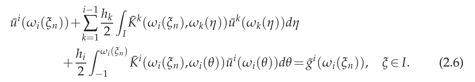
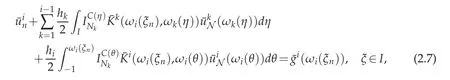
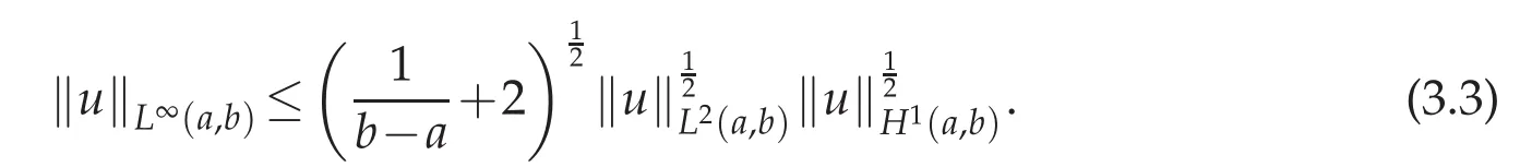
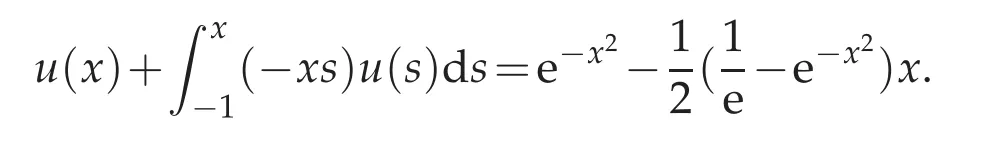
where the given source function g(x)and the unknown function u(x)are supposed to be sufficiently smooth,and K∈C(D)with D:={(x,s):−1≤s≤x

In[4]the Chebyshev collocation method has been proposed to solve the Volterra integral equations of the second kind with singular kernel.

In this paper,we will provide a domain decomposition method in the Chebyshev collocation method for the equation(1.1)and make a rigorous error analysis.The method can avoid errors caused by mapping a large integral interval into very short ones,and computation can be simplified because in each subinterval it can be implemented in a same way.We will split the interval[−1,1]into subintervals,and the more the subintervals are,the faster the computing efficiency is.We use the Chebyshev collocation method which can avoid the appearance of weakly singular weight function ω(x)=The obtained numerical results satisfy exponential rate of convergence,which coincides with convergence analysis.

This paper is organized as follows.In Section 2,we introduce spectral collocation methods and domain decompositions method for the linear and nonlinear second-kind Volterra integral equations.Some basic lemmas are given in Section 3.In Section 4,we present the convergence analysis.And in Section 5,we provide numerical experiments which are used to demonstrate the results obtained in Section 4.

2 The schemes

In this section,we introduce multidomain Chebyshev collocation method for the linear and nonlinear Volterra integral equations.

We split the interval Λ into several subintervals Ii=[xi−1,xi](i=1,2,···,M),where

Let hi=xi−xi−1,ui≡u|Ii,1≤i≤ M.Denote PN(I)be the set of all algebraic polynomials of degree at most N over the interval I=[−1,1],and N is a positive integer.

In the following,we introduce notations

Bywe denote the Chebyshev interpolation operator at the Chebyshev-Gauss-Lobatto (CGL) points xj=cosand it satisfies

Defineas an operator produced by the Chebyshev interpolation operatorwhich obeys

Finally,introduce ξ=by which Equation(2.1)can be written as

2.1 For linear Volterra integral equation

Consider the following linear Volterra integral equation:

On each subinterval we have

It is transferred to an equivalent form defined on the reference interval I,which reads

Then we get the following equation at CGL points ωi(ξn),(n=0,1,···,Ni)of each subinterval Ii,

Assume that Equation(2.5)holds at the collocation points ωi(ξn).We make interpolation for function K(η)u(η)in each subinterval where we letbe the approximation ofThen we obtain the domain decomposition Chebyshev-Gauss-Lobatto collocation scheme of(2.5)

where uN=is the numerical solution of u(x)in whichare the Lagrange basis function associated with the collocation points ωi(ξn)(n=0,1,···,Ni,i=1,···,M).

We then obtain

Next we discuss some implementation issues of the spectral collocation algorithm.Introducing notationsand

GN=

we can write(2.8)as a matrix form:

where matrix A=(Ai,j)is defibed by

for i=1,2,···,M,n=0,1,···,Ni,k =1,2,···,i−1,l=0,1,···,Ni.We discuss an efficient way to computeandwhereis the common j-th Lagrange interpolation basis fuction and ξnis the Chebyshev-Gauss-Lobatto point.In fact,the Lagrange basis function Fj(ξ)can be expressed in terms of the Chebyshev polynomials as the following,

From[13]we have

where

Submitting the aboveajlintoFj(s)yields

Thus we reach

wherecan be achieved by using the relation 2Tl(ξ)namely,

Herethenandcan be evaluated easily.By using this method that we deal with the integral part of the integral equation we can avoid appearance of the weakly singular weight functionω(x)=In[14],the similar numerical integration method we used here can be found.And it was proved both in theory and numerically that the numerical integration method used in[14]is as good as the Gaussian quadrature.In fact,we also get good results both in theory and numerically by using this numerical integration method to solve the second-kind Volterra integral equations.

2.2 For nonlinear Volterra integral equation

Consider the following nonlinear Volterra integral equation

where the source functiong(x)andK(x,s)are sufficiently smooth.Its domain decomposition Chebyshev-Gauss-Lobatto collocation scheme is

whereuN=is supposed to be the numerical solution ofu(x),in whichis the Lagrange basis function associated with the collocation points(n=0,1,···,Ni,i=1,2,···,M).

We then obtain

The above numerical scheme leads to a nonlinear system forSimilar to linear case,we can get its matrix form as follows

whereB(UN)is a function ofUN.We can solve the nonlinear system by a simple iterative method.LetUN=GN−B(UN).Choose a proper initial valueUN,0as the approximation ofUN.Substitute it into the right hand side and get theUN,1as the new approximation ofUN.Repeat this procedure until|UN,k+1−UN,k|<ε.

3 Some basic lemmas

In the following,by k·k we denote the norm of the spaceL2(I),

where

Form>0,letHm(I)be the classical Sobolev space equipped with the normk·kmand the semi norm|·|m.

Introduce a piecewise Sobolev space

with the semi-norm

LetCbe a generic positive constant independent ofhi,Niand any function.Sethmax=max1≤i≤Mhi,Nmin=min1≤i≤M(Ni).Next,we give some useful lemmas.

Lemma 3.1.(Sobolev inequality,[15],p.490)For any u∈H1(a,b),the following inequality holds

Lemma 3.2.([17],p.874.)If u∈Hσ(I),σ≥1,then

Lemma 3.3.([16],p.118.)If v∈Hσ(Ii),(σ≥0),then

Lemma 3.4.If u∈(I)(σ≥1),then

Proof.We have from(3.4)and(3.5)that

which gives the desired result.

Lemma 3.5.(Gronwall inequality,Lemma3.4of[6])If a non-negative integrable function E(t)satisfies

where G(t)is an integrable function,then

4 Convergence analysis for nonlinear Volterra integral equation

In this part we analyze the discrete scheme(2.12)of the nonlinear Volterra integral equation and derive the error estimate inL∞norm of the method.

Theorem 4.1.Let u(x)be the exact solution of nonlinear Volterra integral equation(2.11)and assume that

is the numerical solution of u(x)where(x)is the Lagrange basis function associated with thecollocation points(j=0,1,···,Nii=1,···,M).SetN=(N1,···,NM).If u∈Hm(I)and φ(x,u)satisfies a Lipschitz condition with respect to u on I,i.e.,

where L>0is the Lipschitz constant,then for any integer m≥1,

where C is a constant independent ofand

Proof.Multiplying both sides of(2.12)byand summing upnfrom 0 toNiandifrom 1 toMyields

where

is the collocation point anduNis defined by(4.1).Define

Assume that the kernel functionK(x,s)is smooth sufficiently which leads to them-th partial derivative ofK(x,s)to be bounded.

From(4.4)and(2.11),we can obtain

Therefore

where

Then it follows that

Now,letand from Lemma 3.4 and Lemma 3.1 we have

Meanwhile,in(4.7),we have

where

It can also be derived from Lemma 3.4 and Lemma 3.1 that

and

Therefore,we get

Next,

where

Then we can have that

Therefore

J5can be written and estimated as

where

According to Lemma 3.4 and Lemma 3.1,we have

Substituting J1∼J8into(4.7),it obtains that

Then we have

According to the Gronwall inequality(Lemma 3.5),we can get

From all the above estimates together with(4.20),we obtain(4.3).This completes the proof.

5 Numerical example

In this section,we provide some numerical examples,which show that the domain decomposition Chebyshev Collocation Method is efficient and exponentially convergent for both linear and nonlinear Volterra integral equations.

5.1 Linear examples

Example 5.1.This example is about a linear Volterra integral equation of second kind,which is

The exact solution is u(x)=e4x.

Example 5.2.The second example is the following linear integral equation:

It has an exact solutionu(x)=e−x2.

We apply the numerical scheme(2.8)to Example 5.1 and Example 5.2.Maximum absolute errors of these two examples with differentMare displayed in Figure 1 and Figure 2,which indicate that the desired spectral accuracy can be obtained.We also make a comparison for the numerical results of single domain method and multi-domain method.

Figure 1:Maximum errors of Example 5.1

Figure 2:Maximum errors of Example 5.2

5.2 Nonlinear examples

Actually,a lot of Volterra integral equations are nonlinear.Below we give several nonlinear numerical examples.

Example 5.3.This example is concerned with a nonlinear problem:

with an exact solutionu(x)=exsin(3πx).

Example 5.4.We next consider the following nonlinear Volterra integral equations.

Exact solution of the equation isu(x)=x.

Figure 3:Maximum errors for Example 5.3

Figure 4:Maximum errors for Example 5.4:

Figure 5:Maximum errors for Example 5.5:

Example 5.5.The third nonlinear example is concerned with the nonlinear problem

with an exact solutionu(x)=cos(10x).

Numerical results for Examples 5.3–5.5 can be seen from Figure 3,Figures 4 and 5.Again,it is clearly observed that the errors decay exponentially.The above three examples show that whenNis fixed,the greater the numberMis,the higher convergence order can be obtained.This means we can obtain the high spectral accuracy by splitting the integral interval into more subintervals.

5.3 High oscillating examples

Example 5.6.We consider the following nonlinear Volterra integral equations

whereg(x)=Exact solution isu(x)=cos(λx),which is oscillated whenλis very big.

Figure 6 describes exact solutionu(x)=cos(200x)of this example.

Numerical results for Example 5.6 withX=5,λ=200 can be seen from Figure 7.The method is very effective for high oscillate case.

Figure 6:Exact solution for Example 5.6

Figure 7:Maximum errors for Example5.6

5.4 Longtime calculations

Example 5.7.We consider the nonlinear Volterra integral equation

with exact solutionu(t)=ln(t+e).Maximum errors of the numerical results withX=40 with differentMis shown in Figure 8,which shows that our method can keep high accuracy whenxis bigger.

5.5 Discontinuous problems

Example 5.8.Consider the nonlinear Volterra integral equation with a discontinuous solution,

where

The exact solution is

For the discontinuous case,we split integral interval into several subintervals.For every splitting,the discontinuous point is the endpoint of one subinterval.The computing results are shown in Figure 9.It is indicated that our method is quite vigourous for discontinuous equations.

Figure 8:Maximum errors for Example 5.7

Figure 9:Maximum errors for Example 5.8

6 Conclusions

In the paper we provided a domain decomposition Chebyshev collocation spectral method for solving the second-kind Volterra integral equations.Theoretically,we also got the spectral convergence rate for solving the nonlinear equations.The obtained numerical results coincide with theoretical analysis.In particular,the method also works well for some longtime computaions and discontinuous or high oscillating problems of nonlinear Volterra integral equaitons.

Acknowledgments

The authors are grateful to the referees for the invaluable comments.This work was supported by the National Natural Science Foundation of China(grant number 11571225).

[1]K.Atkinson,The numerical solution of integral equations of the second kind,Cambridge:Cambridge University Press,1997.

[2]H.Brunner,Collocation methods for volterra integral and related functional equations methods,Cambridge:Cambridge University Press,2004.

[3]G.Elnagar and M.Kazemi,Chebyshev spectral solution of nonlinear Volterra-Hammerstein integral equations,J.Comput.App.Math.,76(1996),147-158.

[4]Y.Chen and T.Tang,Spectral methods for weakly singular Volterra integral euqations with smooth solutions,J.Comput.Appl.Math.,233(2009),938-950.

[5]Y.Chen and T.Tang,Convergence analysis of the Jacobi spectral-collocation methods for Volterra integral equations with a weakly singular kernel,Math.Comput.,79(2010),147-167.

[6]T.Tang,X.Xu and J.Cheng,On spectral methods for Volterra integral equations and the convergence analysis,J.Comput.Math.,26(2008),825-837.

[7]T.Tang and X.Xu,Accuracy enhancement using spectral postprocessing for differential equations and integral equations,Commun.Comput.Phys.,5(special ICOSAHOM07 issue)(2009),779-792.

[8]Z.Xie,X.Li and T.Tang,Convergence analysis of spectral Galerkin methods for Volterra type integral equations,J.Sci.Comput.,53(2012),414-434.

[9]X.Li and T.Tang,Convergence analysis of Jacobi spectral collocation methods for Abel-Volterra integral equations of second kind,Front.Math.China,7(2012),69-84.

[10]X.Li,T.Tang and C.Xu,Parallel in time algorithm with specthal-subdomain enhancement for Volterra integral equations,SIAM J.Numer.Anal.,51(2013),1735-1756.

[11]P.Zanolli,Domain decomposition algorithms for spectral methods,Calcolo,24(1987),210-240.

[12]C.Sheng,Z.Wang and B.Guo,A multistep Legendre-Gauss spectral collocation method for nonlinear volterra integral equations.SIAM J.Numer.Anal.,52(2014),1953-1980.

[13]J.Shen and T.Tang,Spectral and high-Order methods with applications,Science Press,Beijing,2006.

[14]L.Trefethen,Is Gauss quadrature better than Clenshaw-Curtis?SIAM Review,50(2008),67-87.

[15]C.Canuto,M.Hussaini,A.Quarteroni and T.Zang,Spectral methods scientific computation:fundamentals in single domains,Berlin:Springer-Verlag,2006.

[16]P.Ciarlet,The finite element method for elliptic problems,Amsterdam:North Holland,1978.

[17]H.Ma,Chebyshev-Legendre spectral viscosity method for nonlinear conservation laws,SIAM J.Numer.Anal.,35(1998),869-892.