Karhunen-Love Expansion for the Discrete Transient Heat Transfer Equation

Tarik Fahlaoui

Sorbonne Universit s,UTC,EA 2222,LMAC,F-60205 Compi gne,France.

1 Introduction

In many applications,we compute the same partial differential equation with different parameters.For instance,let us assume that we want to find the more adequate material to our target application.In order to do so,we run a simulation of the PDE in which the material is represented by one or several parameters,changing for each computation these parameters.However,computing the solution each time is costly.We could construct a basis with a much smaller dimension than with a regular method,by choosing solutions with special parameters.The reduction of the dimension is theoretically ensured by the exponential decay of the KolmogorovN-width,for linear PDEs and some non-linear PDEs(see[29]).This result allows us to find the solution to our PDE in a space of dimensionNsuch that the error between the solution of this equation and the approximate solution computed with the reduced basis decreases fastly withN(see[6],[16]for more details).Two main methods are usually used:thegreedy methodwhich consist in constructing a hierarchical basis provided by an estimate error(see[15]),and theProper Orthogonal Decomposition(POD)which compresses a set of snapshot(solutions to the PDE for fixed parameters)to withhold the main information(see[16],[17]).For parametric PDEs,we can show that the performance of thegreedy methodis related to the KolmogorovN-width(see[16]).

In this article,we focus on Time-dependent equations,for which a POD basis can be constructed.The idea remains the same:provided some snapshots(which can be solutions at either different time steps or different space points),we perform aSingular Value Decomposition(SVD)on the correlation matrix.This compression method appears in many fields under various names such asPrincipal Components Analysis(PCA)in data analysis(see[14]),orKarhunen-Lo ve expansionin statistics to compress a stochastic process([3]).The error estimation of the POD in the literature shows that the performance of this method is related to the decay of the eigenvalues of the correlation matrix([25]or[26]).For experimental temperature fields,a POD was performed and analyzed in[27].However,there is no proof on the decay rate of the eigenvalues.In[28],they explicit this decay by using the smoothness of the solution.Nevertheless,in[1]for bi-variate functions,and in[5]for the heat transfer equation,by using some algebraic properties satisfied by the spatial correlation matrix,they obtain an exponential decay.

For anisotropic parameters or in dimension greater than 1,the analytic solution of the PDE is not accessible.Based on the analysis made in the continuous case,we construct a Karhunen-Love expansion for a discrete solution and show the efficiency of the method by analyzing the decay of the eigenvalues.

We first construct the Karhunen-Love expansion for a discrete solution.We then focus in Section 2 on the transient heat transfer equation discretized in time by two wellknown numerical schemes.By expanding the discrete temperature field in the basis form by the eigenvectors of the Laplace operator,we give an estimate on the error between the temperature field and the truncated KL-expansion.We adopt a new point a view in Section 3,by using the algebraic properties satisfied by the Krylov matrices with Hermitian arguments.Section 4 is dedicated to numerical results:some computations of the eigenvalues to support the theoretical analysis made in Section 2,and an application of this work to the identification of parameters when the data are disturbed by a Gaussian white noise.

1.1 The Karhunen-Lo ve expansion for discrete solution

Let us consider a discrete temperature field in timeTn,represented by a vector of sizeNtsuch that each component belongs toL2(Ω).For each step time,the only assumption on the functionTn(x)is to belong toL2for the space variable.Yet,when we solve a PDE or when we work with experimental data,the solution is discrete in space.However by using an interpolation function,we are able to define the solution as aL2function.Our goal is to compress the data in order to keep only the essential information.In other words,we want to find a basis of small dimension which minimize theL2-error between the discrete temperature field and its projection on this basis.The construction of this basis is well-known under the name of Karhunen-Love expansion,and it has been handle in the continuous case for bi-variate functions([1]).In discrete case,some issues arise and the goal of this paragraph is to construct a Karhunen-Love expansion for discrete function and analyze the performance of this compression method.When we work with discrete time,the first thing is to handle integration in time.Several quadrature rules allow this.In order to remain general,we don’t fix the quadrature weight and just set two numbersξ0andξ1such that

Providing this quadrature rule,we can now define an inner product on RNtwhich can be viewed as the analogous of theL2inner product in the continuous case.It should be noted that the two weightsω0andω1have to be non zero.An example of quadrature rule is given by the trapezoidal rule for whichWe have now all the tools to construct our Kahrunen-Love expansion.Before beginning the construction,let us say some words on the link between the Karhunen-Love expansion presented here and the Singular Value Decomposition(SVD)applied on the matrix storing the degree of freedom,in the case where the temperature field is computed by the finite element method.Assuming a matrix T whose raw components are the degree of freedom(or the value at the grid point)and the line components correspond to the time step.Thanks to the regularity of the solution,we could hope to obtain almost as much information by storing fewer data.A way to keep only the main information is to compute the right and left singular vectors and the singular value ofT.This allows us to obtain T=VΣΦT,whereVis the matrix of the left singular value(corresponding to space)and satisfiesVTV=Id,Φ is the matrix of the right singular value(corresponding to time)and satisfies ΦTΦ=Id,and Σ is a diagonal matrix containing the singular value.An other formulation can be:And since the temperature field is known to be regular,we can hope to have a fast decay of the singular value.An inconvenient of the SVD is that it give us singular vector that are orthonormal for the identity matrix while if the solution is obtain by the finite element method,we would expect the left singular vector to be orthonormal for the mass matrix.And equivalently the right singular vector to be orthonormal for the inner product introduced previously.For this reason we introduce the Karhunen-Love expansion.We first construct the KL-expansion,by introducing some integral operator.And then we show how the performance of this expansion is related to the decay of the singular value.

As mentioned before,we equip the space RNt+1with the inner product(·,·)ωdefined by

in the following,we consider a vectorω∈RNt+1such thatω0=ξ0,ωn=ξ0+ξ1for 1≤n≤Nt−1 andωNt=ξ1.Thus we can rewrite the inner product under the condensed form

We first define the operatorBhby

Roughly speaking,this is the matrix-vector product in continuous case,for a matrix which line components are the step time and the row components stand for the space dependence.As evoked previously,we can work with the singular values and the singular vectors of the operatorBh.However we prefer to work with an auto-adjoint operator in order to use the Spectral theorem.By definition,the adjoint operatoris

We then define the auto-adjointAh:=

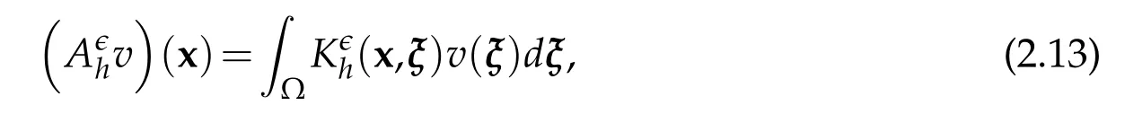
Write under this form,the kernel ofAhisKh(x,ξ):=ωnTn(x)Tn(ξ),and thusAhis an integral operator([18])and so a compact operator.By applying the Hilbert-Schmidt theorem,Ahadmits eigenvectorsvkwhich form an Hilbert basis ofL2(Ω)and are related to non-negative eigenvaluesλk.Finally,Mercer’s theorem([12])allows the following representation ofKh

The final result of introducing this operator is that we can writeTnunder the following form

whereσkstands for the singular value of the operatorBh(or equivalently the square root of the k-th eigenvalue ofAh),andis the projection ofTnon the eigenvectorvk.And the two basisare respectively orthonormal for theL2-product scalar and the discrete product scalar<·,·>ω.

The aim of the KL-expansion is to compress the information.Here we deal with some snapshots of temperature at different time steps. The natural issue is to give an estimation of the truncation error.Let us defineas the truncated function of expression(1.1).We can then show the following classical result in literature.

Proposition 1.1.

Proof.The proof is obvious by using the orthonormality of the eigenvectorsand

Thus,the quality of the KL-expansion is related to the fast decay of the eigenvalues of the operatorAh.In other words,we have to study the spectrum ofAh.We can analyze directly the eigenvalue problem since we have

Unfortunately,we are not able to solve this system set in this form.The first way to rewrite the problem in a more suitable form is to expand each function(Khandv)in an orthonormal basis ofL2(Ω).Thus,the integral over Ω disappears and we can work with an infinite matrix,whose eigenvectors are the coefficients of the eigenvectors ofAhin the orthonormal basis.The natural basis to expand the temperature field is the basis composed of the eigenvectors of the Spatial operator over whichTnis computed.In the next section,we consider the transient heat transfer equation and give an expression of the matrix on which we expect to show the fast decay of the eigenvalues.

2 The governing equation

Let us consider classical assumption such that Ω is an open bounded domain in Rdwith smooth boundary∂Ω,b>0 corresponding to the final time.The equation is defined by

where the unknownTis the temperature field,which belongs toThe diffusion termγis a symmetric and positive tensor,andβis a scalar and represents the heat transfer coefficient.Finally,we assume the right hand sideSto be a separated function on time and space,i.e.

However,in practice the solution to equation(2.1)is just known point-wise in time.We then begin to present an analysis in a discrete context.A first choice when we are interested in computing equation(2.1)is the numerical time scheme.In order to understand the importance of this choice,we consider two well-known schemes which are unconditionally stable.

2.1 Backward Euler scheme

The first scheme we work with is the Backward Euler scheme,which is

withN∆t=b.

According to the Spectral Theoremwe can rewriteTnin the orthonormal basis formed by the eigenvectorsof the Laplace operator K:=−∇·γ∇+β.Thus,expanding the discrete temperature field in this basis gives us

We expand the spatial part ofSandain a similar way.

An advantage to use the basisis that it satisfies the steady heat transfer equation and thus we can give an explicit expression fordepending only onak,θn,fkand the eigenvalues of K which we denote byrk.Straightforward computations over the equation(2.2)yield the following expression forTn,

whereis the inverse ofUsing the definition of an inverse and the eigenvalue problem satisfied by the couplewe have

and finally multiplying this equation byekand integrating over Ω,we obtain the following expression of

whereck=

2.2 Crank-Nicholson scheme

Let us now examine the expression ofwhen the equation(2.1)is discretized by a Crank-Nicholson scheme,given below

We can writeTnas

and using(2.3)and(2.4),it yields

whereck=

We first give the main result of this section,which is the performance of the Karhunen-Love expansion.

Theorem 2.1.Let Tnbe a discrete temperature field computed by the Backward Euler scheme or the Crank-Nicholson scheme.is the M-truncated temperature obtained by the Karhunen-Lo ve expansion,i.e.

Then we have

where C1just depends on Ntand ωn,and νis not greater than18and depends on the initial condition and the source term.C2depends on ν,rk,Nt,∆t,the weights ξ0and ξ1and the initial condition and the source term.

Remark 2.1.This result shows the exponential performance of the Kahrunen-Love expansion.The first term of the RHS is the price of acting with finite matrices.However,it does not reduce the result since we can find ǫ such that this term is negligible with respect to the second term.

Before proving Theorem 2.1,we rewrite the eigenvalue problem(1.2)under a more suitable form thanks to the decomposition(2.5)and(2.7)of Tn.Recalling that Ahis define by

we can expand Khand v inin order to eliminate the integral over Ω.Considering G the matrix which contains the coefficient of the kernel Khinthe operator Ahcan be written

The next step is to use this expression in the eigenvalue problem,multiplying by ekand integrating over Ω and we recover a matricial eigenvalue problem.Here we just define Gas the matrix containing the coefficients of the kernel,by use of(2.5)and(2.7),we can give an explicit form of this matrix.We recall that the kernel Khis defined as

Thus,it is easy to see that the matrix G is defined by

In order to work with temperature field provided from a Backward Euler scheme or a Crank-Nicholson scheme,we set

and we set

Thus for the two schemes,has the same form

The next step is to introduce the expression ofin the expression(2.10)of the matrix G and remove the sum overn.Using the properties of geometric series and switching the sum overiandn,we have the following expression for G.

This form has the advantage of separating the terms of subscriptskandl,except for the factorwhich can be useful as we show later.In the last line corresponding to the product of the RHS terms,the term indexed bykandlare not separated.To avoid this problem,we have by symmetry

and we can finally write G over a form that allows us to analyze it.

The proof of this theorem will be acted in four steps.We first prove that working with finite matrix does not change the result,then we state that the truncated matrix of G satisfies a Lyapunov equation with a displacement of low rank.We give an upper bound on the Zolotarev number of the spectrum of the Lyapunov operator, and we finally conclude with an upper bound on the first eigenvalue of the truncated matrix ofG.

All the previous analysis was dealt with an infinite matrix G.Unfortunately,there are only few results on eigenvalues for infinite matrices.However we can cope with this problem.By assumption,the temperature fieldTnbelongs to the spaceL2(Ω)and using the orthonormality of the basis?ek?(the eigenvectors of the Laplace operator),we can conclude that

If this result does not allow us to cut the matrix G,it gives us an estimation of the error provided by the truncation of the matrix G.Indeed,let the truncated sumTn,N(ǫ)=(x)and the truncated sumintroduced in proposition(1.1),then we have

For the first term in RHS,we chooseǫin such a way that it is negligible and the second term will be handled in proposition(1.1)and the analysis of the cut matrix of G.A more elegant way to show that working with finite matrices does not change the result,is to study the difference between the eigenvalues of the operatorAhand the eigenvalues of the cut matrix of G.Let us introduce the operator:L2(Ω)7→L2(Ω)such that

where we define the kernelas

andUnder this notation,the operatorcorresponds to the finite eigenvalue problem,i.e.the matrix resulting from the decomposition ofin the eigenvectors of the Laplace operator is nothing else than the truncated matrix of G.The operatoris also a compact auto-adjoint operator.Moreover,sinceTn(x)belongs toL2(Ω),the operatorAhandbelongs to the trace class operator.In order to measure the difference between the eigenvalues ofAhandunder the assumption(2.11),we use the perturbation theory for compact operator.Thus we define the operatorE=Ah−.It is also an auto-adjoint operator and we have

We have then the following inequality([24]and[23])

and since||E||≤Tr(E),we have the following estimation

withThis statement tells us that if we cut the matrix G far enough for the assumption(2.11)to become true,then the error between theN(ǫ) first eigenvalues of the operatorAhand the eigenvalues of the truncated matrix is of the orderǫ.

Remark 2.2.The decomposition of the temperature field in the basis formed by the eigenvectors of the Laplace operator,is a theoretical process.Thus we can takeN(ǫ)as large as needed to recover the assumption(2.11).For the computation,we use an other basis to expand the temperature field.IfTnis computed by the finite element method,we choose the shape function.And thus we get the following eigenvalue problem:

whereMdenotes the mass matrix and G the coefficient ofKhin the shape function.Using the Cholesky factorization for positive semi-definite matrixand settingthe eigenvalue can be written

which is aNdof×Ndofeigenvalue problem,whereNdofis the number of degree of freedom.

To make the notation less cluttered,we assume that the matrix G is a finite matrix,i.e.we fix an integerK∈N∗and assume that G∈RK×K.We have a first statement onG:

Proposition 2.1.The matrix G can be written as a Hadamard product between a matrix,diagonally congruous to a matrix P,and a sum of tensor product of vector,i.e.

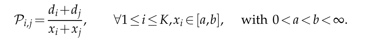
where the matrix P is defined by

Proof.Settingand∆=diagyields

and since we have written G in a way that all terms are separated,the result follows.For the Backward Euler scheme,The eigenvaluesgrow to infinity and are positive,thus we have:r1≤...≤rK.And thus

For the Crank-Nicholson scheme,we havea=

Remark 2.3.Hereνdepends on the initial state and the RHS.If neither of them is identically zero,thenν=18.If the RHS is zero,ν=4 and ifa=0,ν=6.As we will see later,νcorresponds to the rank of the matrix G.Roughly speaking,the smoother the solutionTnis,the smallerνis.It is then natural that this number depends on the operator K,the initial state,and the RHS.

This expression for G will be useful in order to show the fast decay of its eigenvalues.Indeed,the matrix P is a Pick matrix([4]),which appears in interpolation problems,except that the coefficientxican be equal.Thus,we can write a Lyapunov equation on which P is the solution.And we will use this equation to show the exponential decrease of G’s eigenvalue.We first begin by showing that G is solution to a Lyapunov equation:

Proposition 2.2.The matrix G satisfies a Lyapunov equation with a displacement of rankν,i.e.

whereDx=

Proof.Using the expression(2.1),we can rewrite G by

with the notationDαi,1=diag(αi,1).The next step is to show that P satisfies a Lyapunov equation by using the Kronecker product and thevec-operator.Let us setDx=diag(xi),with the coefficientxidefined above.We have

Multiplying byvec(P),it yields

and finally P satisfies the following Lyapunov equation([19])

We setin the previous proposition,so that

By commutative properties of the multiplication of two diagonal matrices and summing overiwe find the result.

Proposition 2.3.The eigenvalues of the matrix G have an exponential decay,i.e.

Proof.In Proposition 2.2,we have shown that G satisfies the Lyapunov equation

whereDx=diag(xi)and ∀1≤i≤K,xi∈[a,b]with 0

whereZkis the Zolotarev number.And finally using the upper bound[2,Corollary 3.2.],we have

which concludes the proof.

We can express the exponential decay of the eigenvalues of G as

which gives us the upper bound in Theorem 2.1,where we begin atMthe sum overk.

Remark 2.4.The exponential decay is related to the value ofwhich is nothing else thanκ(Dx),the condition number of the matrixDx.Ifκ(Dx)tends to infinity,we lose the exponential convergence.In the case where the RHS is equal to zero,the Lyapunov equation satisfied by G becomes

withB∈RK×4.SinceDxhas eigenvalues contained in a strip around the real axis and is diagonal,we have the following decay for G whenκ?Dx?tends to infinity([20])

When the RHS is non zero,we don’t have a similar result,however the decay of the eigenvaluesremains exponential for largeK(for more details refer to[1,Remark A.1.]).

When we explicit the quotientfor each time scheme,we see that it is related to the quotient between the maximal and minimal eigenvalues of the Laplace operator.Indeed,we havefor the Backward Euler scheme andfor the Crank-Nicholson scheme.

When we construct our matrix G,we fix an integerKin order to work with finite matrix.And since the sequencegrows to infinity,the quotientgrows withK.

Thus,the upper bound(2.16)ensures the exponential decay of the eigenvalue,even if the decay is slow.This issue will be supported by numerical experiment in Section 5.

We have then show that working with finite matrices yields an error which can be control to be negligible,and we show the exponential decay of the eigenvaluesWe finally give an upper bound of the first eigenvalue

Proposition 2.4.The first eigenvalue of G can be bounded as

Proof.Sinceλ1(G)≤||G||F,we have to give an upper bound of the Frobenuis norm of G.From(2.15),we have the following form for G

Thus,we have Using the fact that the eigenvalues of the Laplace operator grow to infinity.And finally,setting C=gives us the expected result.

The Theorem 2.1 shows the performance of the Karhunen-Love expansion applied to the discrete heat transient equation.However the KL-expansion was constructed by using the operator Ah:L2(Ω)7→ L2(Ω).Assuming that the data are provided by a finite element method,we have a matrix T which stores the degree of freedom at each time step.Computing the eigenvalue problem Ahvk=λkvkis equivalent to computing an Ndof×Ndofeigenvalue problem.But if we define Ahas Ah=Bhthe eigenvalue problem’s size becomes Nt+1×Nt+1 which can be expected to be much smaller.This arises the following issue:does the KL-expansion remain good?And as stated in this section,it is equivalent to determine if the eigenvalues have an exponential decay.An other issue is the case of noisy data.Intuitively,there is no reason to expect an exponential decay since adding a white noise to the data amounts to add information.To tackle such questions,we will work directly with the singular value problem:Bhvk=σkφk.

3 A more general approach:Krylov matrices with Hermitian argument

As made in the previous section,we begin by constructing the matrix on which we made the singular value decomposition.We recall the definition of the operator from which we constructed the KL-expansion.

The operator Bh:L2(Ω)→RNt+1is defined by

His adjoint operatoris defined from RNt+1→L2(Ω)by

We are interested in the singular value problem

This singular value problem can be viewed as the continuous case of the singular value decomposition applied to the matrix T which stores the data.As we will later see,the singular vectors computed are orthonormal for a matrix which can be different to the identity.

To write the matrix under a suitable form,we will assume that there exists an orthonormal basis ekof L2(Ω)such that the coefficients of the discrete temperature field in this basis have the following form

Where K1andK2are Krylov matrices with Hermitian argument,i.e.of the formwhere A is a square Hermitian matrix and x a vector.We assume also that Θ is invertible.

Remark 3.1.From(2.9),the coefficients of Tnin the basis formed by the eigenvectors of the Laplace operator are

If we setwhere Dc=diag(ck)and a=(ak),and finally

we recover the general form.Note here that Θ is not invertible,however noting thatwhereandsuch that γ+6=0,we can recover the form(3.3).

We can now construct the singular value problem by putting the expression(3.3)ofin(3.1)and(3.2).It yields

and similarly

Thus we get

and multiplying byeland integrating over Ω the expression ofB∗,it yields

To make the notation less cluttered,we define the matrix T by Tk,n=

Note that it is nothing else than the coefficient ofTnis the basisek.At the end,the matrices are written

LetL=diag(ωn),we have

Settingψk=it yields

and finally

Thus we have just to focus on the singular values of the matrix

Remark 3.2.Ifare the eigenvalues of the Laplace operator,we get:

And similarly,the eigenvalue problemBB∗φ=λφexpanded in the basiswill be

where we recallψ=

3.1 Exponential decay

In order to recover the exponential decay of the singular valueswe take advantage of the Krylov matrices,which singular values have an exponential decay.An example of Krylov matrices are the well-known Vandermonde matrices.However,as in the first section,we have to deal with finite matrices,and thus we assume T belonging to RK×Nt+1.We finally recover an error estimate as the one given in Theorem 2.1,by the upper bound(2.12).

We begin this section by giving the main result:

Proposition 3.1.Assuming the number of time subdivisionsNtis odd,then the singular values ofTdecrease as such

whereθnare the diagonal coefficients of the matrix Θ.

Remark 3.3.The assumptionNtodd is not essential.IfNtis even,the formula remains unchanged except for the numerator in the exponential,which becomes

Before beginning the proof,we can remark that the constant in the log term only depens onNtwhich have no reason to tend to infinity.

Proof.The proof will be made in three parts.We first state the exponential decay for the singular value of a Krylov matrix,then we show the exponential decay ofandby the Courant-Fischer theorem,and finally we conclude by the additive Weyl’s theorem.

Let Kk,n=Krylov matrix with Hermitian argument(i.e.A is an Hermitian matrix).

It yields([2,Corollary 5.2])

where[N]2is zero ifNis even and 1 otherwise.By the Courant-Fischer Theorem([21,p.555]),we know that

whereGkdenotes the set of all vectorial subspace of dimension equal tok.For the first singular value we have then

and then by setting y=it yields

since||y||2=1.For the second singular value,we have

Setting again y=y belongs to V′and||y||2=1,thus we have

And since it is true for all V′∈GNtpassing to the min,it yields

Doing the same for each k gives

And similarly we have

Finally,by the additive Weyl’s inequality([11]),we have

which concludes the proof.

The Proposition 3.1 shows the performance of the KL-expansion in the case where we solved the eigenvalues BB∗φ=λφ or B∗Bv=λv.When we have our eigenvectorsin the first case orvkkin the second case the next step is to project the temperature fields into the basis form by these eigenvectors,i.e.in the first casevwill be defined by

kkvk(x)=

An advantage to work with the singular value problem is to avoid this projection step,indeed performing a singular value decomposition on the matrixgives usσv,and we have just to computewhere we recall

When the data are provided by an experiment,there are disturbed.We frequently add a Gaussian white noise to the solution to numerically reproduce this phenomena.Thus we analyze the decay of the singular value when the temperature field are disturbed.

3.2 Disturbed data

Let consider Tnas in the previous section.We consider a Gaussian white noise ǫn(·)with variance denoted by σ2.The disturbed temperature fieldis defined by

By assumption(3.3),we know that the coefficients of Tnin an orthonormal basisof the space L2(Ω)are

Similarly,we can expand ǫn(·)in the basisi.e.

whereAnd finally the coefficients ofare given by

In the previous section,we have constructed our singular value problem which waswhere the matrix T was nothing else than the one containing the coefficients of Tnin the basisHere we have to take account of the noise,and so we denote bythe new matrix.The new singular value problem becomes

where we denote E by

We have then the following result.

Proposition 3.2.The singular values of the matrixare as such

where we have

and P is the orthogonal projection onto the column space of

Proof.By construction,we have

The result follows by[22].

Since the spectral norm ofis related to σ2such thatthe Proposition 3.2 tells us that the singular values for the disturbed temperature field have a decay similar to the singular values for the non-noisy temperature field while the variance σ2is inferior to the singular values.In other words,when the singular value corresponding to the non-disturbed temperature field is less than the variance,the decay stops to be exponential.This result will be supported by numerical computations in the next section.

4 Numerical computations

4.1 Eigenvalues of the operator A=B∗B

The performance of the KL-expansion is related to the fast decay of the eigenvalues(or singular values)as stated by Proposition 1.1.In the first section,we prove that this decay is of the form

This result allows us to conclude on the fast decay of the eigenvalues,however a special interest should be taken in the constantIndeed,iftends to infinity,the constant in square brackets tends to 1 and so we lose the fast decay.Fortunately,when this quotient tends to infinity we keep an exponential decay with a square root exponent for a zero RHS,i.e.

and we can also show that we keep an exponential decay for a non zero RHS.To illustrate that,we consider the one dimensional case,where the eigenvalues of the Laplace operator are known.Let consider the following equation

In this case the eigenvalues of the Laplace operator are rk=αk2+β.In order to work with finite matrices,we have chosen an integer K large enough so that the error committed byusing finite matrices does not affect the result.For a Crank-Nicholson time scheme,we have

Figure 1:The initial state corresponding to the Fourier coefficients for a truncated number K=21.

Similarly,

for the Backward Euler scheme.It is clear thatb/agrows withK.

In the two cases,we expect that the eigenvalues decrease less quickly whenKgrows.We consider the initial state defined by

Thus,the initial state belongs toL2(Ω)and have no more regularity.We cut the sum overktoKfor different value ofKand display the eigenvalues of the matrix G,whose coefficients are given by(2.10).The functionT0truncated forK=21,is depicted in Fig.1.

The final time is fixed tob=0.1 and the time step is 10−3.We use the trapezoidal rule for the time integration.The thermal coefficientsαandβare fixed to 1.In Figure 2 we represent the twelve first eigenvalues ofAfor differentK.

The eigenvalues seem to decrease to zero exponentially even ifKbecomes larger,which is consistent with the upper bound(4.2).We now consider a non zero RHS.For this purpose we define the separated functionSby

Figure 2:Eigenvalues of G for a zero RHS,K varies from 15 to 100,for the Backward Euler scheme(left)and the Crank-Nicholson scheme(right).

Figure 3:Eigenvalues of G for a non zero RHS,K varies from 15 to 100,for the Backward Euler scheme(left)and the Crank-Nicholson scheme(right).

And we compute the eigenvalues of G as shown above.The decay of the eigenvalues is depicted in Figure 3.

The eigenvalues decrease exponentially even ifKgrows.

4.2 Identification problem

We now present an application of the Karhunen-Love expansion constructed and analyzed in this article.Let us suppose that we have a temperature field(Tn)0≤n≤Nwhich is obtain numerically with a Backward Euler scheme or a Crank-Nicholson scheme for the time approximation and the finite element method with Lagrangian basis of degree 1 for the space approximation.In this case the temperature field is known as a matrixT,such that the columns are vectors containing the values of the temperature field at the mesh points,which is consistent with the data measured by a camera.The final goal is to recover the parameters(α,β).However,in practice,some noises appear due to the camera’s defects.We can then construct the following matrix with artificial noise

where ǫi,jfits with the difference between the real temperature and the temperature measured by the camera.Thus,ǫi,jwill be small for a camera with a high precision.To recover the thermal parameters,we write the equation under the variational formulation and expand the solution by using the Karhunen-Love expansion.Hence,we obtain more equations than unknowns.However,since the temperature fielddoes not solve the discrete heat equation,we have an ill-posed inverse problem.We must then choose few equations and use a least-squares method.The Karhunen-Love expansion then allows us to keep the equations with the most information.This issue was handled in the continuous case in[5,7–9].

4.2.1 Karhunen-Love expansion

We begin by just considering the perturbed matrixand forget how it is obtained.If we construct our Karhunen-Love expansion by expanding the temperature field in the shape functions,it yields

where M denotes the mass matrix.As shown in the Section 4,we set ψ =φ and w=where we use the Cholesky factorization for semi definite symmetric matrices(M=We then obtain

Thus,we can apply the classical Singular Value Decomposition

If we construct the matrix V=we get the coefficients of the eigenvectors vkin the shape functions.Thus,vk(x)=Moreover,where Φ=Hence,we obtain the Karhunen-Love expansion

This expansion allows us to represent the temperature fieldby a sum of few elements with a small error since the singular values of B decrease fastly to zero.For numerical example,we just consider the case of a Backward Euler scheme.We thus compute

Figure 4:(left)Singular values of B.(right)Truncation error in norm L2and in semi-norm H1.

the singular values ofBas explained before,and compare them to the error made by the truncated sum in the discrete anisotropic norms

For the computation,we fix(α,β)=(1,1),S(x,t)=with the numbers of time points and space points equal to 101,and the initial time defined in(4.4).We first present this result when the variance is zero as shown in Figure 4.

This result show that the exponential decay of the eigenvalues leads to an exponential decay of the error.This is in accordance with the proposition 1.1 for theL2-norm.For the semiH1-norm we can deduce a similar result

whereris the minimum between the number of time point and space point.By summing overnit yields

by the orthonormality offor the weighted inner product(φ,ψ)ω=Moreover,the eigenvectorsbelong to H1(Ω)([5,Proposion 3.1]),thus the quantity maxk∈{M+1,r}|vk|H1(Ω)is finite.

We now examine the case where the variance is non-zero.We compute the singular values for different variances,and display the incidence on the truncation error in Figure 5.

The reason why the singular values have no exponential decay comes from the Proposition 3.2.We have the following link between the singular values for a temperature field with and without noise

where ξkand ηkdepend of the variance σ2.Intuitively,the exponential decay of the singular values shows that the information contained in the matrix˜Tis poor.The exchange of heat is a smooth phenomenon,the variation of temperature near two time points or two space points is small.However,when we add some noise we change the regularity of the solution and we add a lot of information.It is then reasonable to lose the exponential decay of the singular value.

4.2.2 Time-Space equation

Let us return to the identification problem.We identify the parameters thanks to the equation(4.3)discretized by a Backward Euler scheme,i.e

To reach this point,we proceed in two steps.The first one,assuming the temperature field to be non disturbed,is to write the equation satisfied by the parameters and by a least-square method to recover the parameters.Note that since the temperature Tnis the exact solution to our problem,we recover the parameters exactly.As a second step,we use the disturbed solutionand solve the equation by using the least-squares method as if the temperature field was non disturbed.In this case,an error is committed sinceis not solution of(4.7).However,we are hoping to keep the most information by using the KL-expansion.

Assuming the temperature field to be computed by a FEM method and not disturbed by a Gaussian noise.Considering equation(4.7)in a weak form,we get

The next step is to use the Karhunen-Love’s expansion of(Tn)nand set u=vl(vlbelongs toH1(Ω)by[5,Proposion 3.1]).By the orthogonality of(vk)kwe get

Figure 5:(left)Singular values of B,the circle corresponding to a zero variance,and the triangle corresponding to the case where the variance vary from 10−4to 0.1.(right)The truncation error in norm L2and H1for non-zero variance(triangle),and zero variance(circle)

Setting(DΦ)n+1,l=Kthe stiffness matrix,andsuch that

we have the following equation

where Φ andVare the singular vectors defined in(4.6),and Σ the diagonal matrix of the singular values.We set

By equation(4.8),the identification problem can be expressed as finding a couplesuch that

We then search the couple which minimizes this quantity.And settingandwe get two equations for two parameters.However,when we consider the full matrix H(α,β),the least-square procedure can fail because of the size of the matrix,even if we consider a non disturbed temperature field.In order to fix it,we can consider the truncated matrix HN(α,β),where we take the?N×N?- first term.Truncating the matrix amounts to truncating the KL-expansion,and as viewed above it is a way of keeping the most information with the less amount of data.Thus,using the KL-expansion has a significance in this case.

For numerical computations,we consider two initial states,one singular and a second smoother.In order not to perturb to much the temperature field,we re-scale the initial state and the source term such that the temperature computed by the FEM is close to 100.Here,the Fourier coefficients are respectively given by

We depicte in Figure 6 the two initial states.Intuitively,the singular initial state can be represent with fewer modes than the smooth one.The RHS will beas the one used to show the decay of the singular value.The numbers of time points and space points are fixed to 500,and the domain on which we compute the solution is?0,π?×?0,0.1?.The variance will be varying between 0.01 and 1.Since we add a random matrix,the result can be different from one experience to an other.In order to avoid this variation,the result will be an average of several computations.We take?α,β?=?exp(1),3π?≈?2.72,9.42?as shown in[5].The results are presented in Table 1.For our simulation,we add a noise on the temperature field and perform the Karhunen-Love expansion on the disturbed field.In[5],the noise is introduced in the Gram matrix.The result depicted in Table 1 seems to be less sensitive to the noise than in[5].

Figure 6:(left)Singular initial state.(right)Smooth initial state.

Table 1:

5 Conclusion

This article aims to adapt the Karhunen-Love expansion to the discrete transient heat transfer equation.An error estimate is given based on the exponential decay of the eigenvalues of the spatial correlation matrix.The key point in this paper is the decomposition of the temperature field in the Laplace operator’s eigenvalues,which allows us to conclude on the performance of the Karhunen-Love expansion in the case we consider the spatial correlation matrix.Since the field is assumed to be discrete in time,an other analysis is performed on the singular values.This allows us to show the performance of considering the time correlation matrix which give us a less costly eigenvalue problem to solve since the number of time points is generally smaller than the number of space points.Finally,we show the lack of decay in the case where the temperature field is disturbed by a Gaussian white noise.This is consistent with the fact that the data is enriched.All this results are successfully supported by some numerical experiments.Then,we present a practical way to compute the Karhunen-Love expansion,in the case where the temperature field is computed by the finite element method.Finally the usefulness of the KL-expansion is enhanced by an direct application to an identification problem with noisy data.

[1]M.Azaiez and F.Ben Belgacem,Karhunen Loves truncation error for bivariate functions,Computer Methods in Applied Mechanics and Engineering,290(Supplement C)(2015),57-72.

[2]B.Beckermann and A.Townsend,On the singular values of matrices with displacement structure,SIAM Journal on Matrix Analysis and Applications,38(2017),1227-1248.

[3]A.Alexanderian,A brief note on the Karhunen-Loeve expansion.

[4]D.Fasino and V.Olshevsky,How bad are symmetric Pick matrices?,Advanced Signal Processing Algorithms,Architectures,and Implementations X,4116(2000),147-156.

[5]E.Ahusborde,M.Azaiez,F.Ben Belgacem and E.Palomo Del Barrio,Mercer’s spectral decomposition for the characterization of thermal parameters,J.Comput.Physics,29(4)(2015),1-19.

[6]A.Quarteroni,A.Manzoni and F.Negri,Reduced Basis Methods for Partial Differential Equations:An Introduction,Springer International Publishing,2015.

[7]A.Godin,Estimation sur des bases orthogonales des proprits thermiques de matriaux htrognes proprits constantes par morceaux,Thse de doctorat,Bordeaux 1,2013.

[8]E.Palomo Del Barrio,J.-L.Dauvergne and C.Pradere,Thermal characterization of materials using KarhunenCLove decomposition techniques C Part I.Orthotropic materials,Inverse Problems in Science and Engineering,20(8)(2012),1115-1143.

[9]E.Palomo Del Barrio,J.-L.Dauvergne and C.Pradere,Thermal characterization of materials using Karhunen C Love decomposition techniques C Part II.Heterogeneous materials,Inverse Problems in Science and Engineering,20(8)(2012),1145-1174.

[10]M.Stewart,Perturbation of the SVD in the presence of small singular values,Linear Algebra and its Applications,419(1)(2006),53-77.

[11]H.Weyl,Das asymptotische Verteilungsgesetz der Eigenwerte linearer partieller Differential gleichungen(mit einer Anwendung auf die Theorie der Hohlraumstrahlung),Mathematische Annalen,71(1912),441-479.

[12]J.Mercer,Functions of Positive and Negative Type,and their Connection with the Theory of Integral Equations,Philosophical Transactions of the Royal Society of London A:Mathematical,Physical and Engineering Sciences,209(1909),415-446.

[13]J.B.Conway,A Course in Functional Analysis,Springer New York,1994.

[14]I.T.Jolliffe,Principal Component Analysis,Springer Verlag,1986.

[15]A.Buffa,Y.Maday,A.T.Patera,C.Prud’homme and G.Turinici,A priori convergence of the Greedy algorithm for the parametrized reduced basis method,ESAIM:Mathematical Modelling and Numerical Analysis,46(3)(2012),595-603.

[16]J.S.Hesthaven,G.Rozza and B.Stamm,Certified Reduced Basis Methods for Parametrized Partial Differential Equations,Springer International Publishing,2015.

[17]S.Volkwein,Proper orthogonal decomposition:Theory and reduced-order modelling,Lecture Notes,University of Konstanz,4(4)(2013).

[18]H.Brzis,P.G.Ciarlet and J.L.Lions,Analyse fonctionnelle:thorie et applications,Dunod,1999.

[19]K.Schacke,On the Kronecker Product,2004.

[20]L.Grubisic and D.Kressner,On the eigenvalue decay of solutions to operator Lyapunov equations,Systems and Control Letters,73(Supplements C)(2014),42-47.

[21]C.D.Meyer,Matrix Analysis and Applied Linear Algebra,Society for Industrial and Applied Mathematics,2000.

[22]G.W.Stewart,A note on the perturbation of singular values,Linear Algebra and its Applications,28(Supplement C)(1979),213-216.

[23]K.Fan,Maximum properties and inequalities for the eigenvalues of completely continuous operators,Proceedings of the National Academy of Sciences,37(11)(1951),760-766.

[24]A.Guven,Quantitative Perturbation Theory for Compact Operators on a Hilbert Space.Ph.D Dissertation,Queen Mary University of London,2016.

[25]Z.Luo,J.Zhu,R.Wang and I.M.Navon,Proper orthogonal decomposition approach and error estimation of mixed finite element methods for the tropical Pacific Ocean reduced gravity model,Computer Methods in Applied Mechanics and Engineering,196(41)(2007),4184-4195.

[26]M.Hinze and S.Volkwein,Properorthogonal decomposition surrogate models for nonlinear dynamical systems:Error estimates and suboptimal control,Dimension reduction of largescale systems,Springer,2005,261-306.

[27]R.Ghosh and Y.Joshi,Error estimation in POD-based dynamic reduced-order thermal modeling of data centers,International Journal of Heat and Mass Transfer,57(2)(2013),698-707.

[28]M.Griebel and H.Harbrecht,Approximation of bi-variate functions:singular value decomposition versus sparse grids,IMA journal of numerical analysis,Oxford University Press,34(1)(2013),28-54.

[29]A.Cohen and R.Devore,Kolmogorov widths under holomorphic mappings,IMA Journal of Numerical Analysis,Oxford University Press,36(1)(2016),1-12.