Convergence Analysis of an Unconditionally Energy Stable Linear Crank-Nicolson Scheme for the Cahn-Hilliard Equation

Lin Wang and Haijun Yu

School of Mathematical Sciences,University of Chinese Academy of Sciences,Beijing 100049,China

NCMIS&LSEC,Institute of Computational Mathematics and Scientific/Engineering Computing,Academy of Mathematics and Systems Science,Beijing 100190,China.

1 Introduction

In this paper,we consider numerical approximation for the Cahn-Hilliard equation

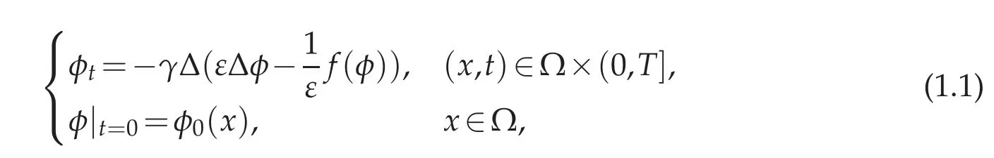
with Neumann boundary condition

Here Ω∈Rd,d=2,3 is a bounded domain with a locally Lipschitz boundary,n is the outward normal,T is a given time,φ(x,t)is the phase- field variable.Function f(φ)=F′(φ),with F(φ)is a given energy potential with two local minima,e.g.the double well potential

The two minima of F produces two phases,with the typical thickness of the interface between two phases given by ε. γ is a time relaxation parameter,its value is related to the time unit used in a physical process.

Eq.(1.1)is a fourth-order partial differential equation,which is not easy to solve using a finite element method.However,if we introduce a new variable µ,called chemical potential,forEq.(1.1)can be rewritten as a system of two second order equations

The corresponding Neumann boundary condition reads

The Cahn-Hilliard equation was originally introduced by Cahn-Hilliard[6]to describe the phase separation and coarsening phenomena in non-uniform systems such as alloys,glasses and polymer mixtures.If the term ∆µ in equation(1.3)is replaced with−µ,one get the Allen-Cahn equation,which was introduced by Allen and Cahn [2] to describe themotion of anti-phase boundaries in crystalline solids. The Cahn-Hilliard equation and the Allen-Cahn equation are two widely used phase- field model.In a phase- field model,the information of interface is encoded in a smooth phase function φ.In most parts of the domain Ω,the value of φ is close to local minima of F.The interface is a thin layer of thickness ε connecting regions of different local minima.It is easy to deal with dynamical process involving morphology changes of interfaces using phase- field models.For this reason,phase field models have been the subject of many theoretical and numerical investigations(cf.,for instance,[7–9,12,14,15,17,19,22,23,30,35]).

However,numerically solving the phase- field equations is not an easy task,since the small parameter ε in the Cahn-Hilliard equation makes the equation very stiff and requires a high spatial and temporal grid resolution.To design an energy stable scheme,one should respect the physical dissipation law of the Cahn-Hilliard system.In fact,the Cahn-Hilliard equation is H−1gradient flow of the Ginzburg-Laudau energy functional

More precisely,by taking the inner product of(1.3)with µ,and integration in time,we immediately find the following energy law for(1.3)

Since the nonlinear energy F is neither a convex nor a concave function,treating it fully explicit or implicit in a time discretization will not lead to an efficient scheme.In fact,if the nonlinear force f is treated fully explicitly,the resulting scheme will require a very tiny step-size to be stable(cf.for instance[35]).On the other hand,treating it fully implicitly will lead to a nonlinear system,for which the solution existence and uniqueness requires a restriction on step-size as well(cf.e.g.[19]).One popular approach to solve this dilemma is the convex splitting method[16,17],in which the convex part of F is treated implicitly and the concave part treated explicitly.The scheme is of first order accurate and unconditional stable.In each time step,one need solve a nonlinear system.The solution existence and uniqueness is guaranteed since the nonlinear system corresponds to a convex optimization problem.The convex splitting method was used widely,and several second order extensions were derived in different situations[5,9,11,26],etc.Another type unconditional stable scheme is the secant-line method proposed by[12].It is also used and extended in several other works,e.g.[4,5,9,18,22,25,29,45].Like the fully implicit method,the usual second order convex splitting method and the secant type method for Cahn-Hilliard equation need a small time step-size to guarantee the semi-discretized nonlinear system has a unique solution(cf.for instance[3,12]).To remove the restriction on time step-size,a diffusive three-step Crank-Nicolson scheme was introduced by[26]and[13]coupled with a second order convex splitting.After time discretization,one get a nonlinear but unique solvable problem at each time step.

Recently,a new approach termed as invariant energy quadratization(IEQ)was introduced to handle the nonlinear energy.When applying to Cahn-Hilliard equation,it first appeared in[23,24]as a Lagrange multiplier method.It then generalized by Yang et al.and successfully extended to handle several very complicated nonlinear phase- field models[27,40–43].In the IEQ approach,a new variable which equals to the square root of F is introduced,so the energy is written into a quadratic form in terms of the new variable.By using semi-implicit treatments to the nonlinear equation using new variables,one get a linear and energy stable scheme.It is straightforward to prove the unconditional stability for both first order and second order IEQ schemes.Comparing to the convex splitting approach,IEQ leads to well-structured linear system which is easier to solve.The modified energy in IEQ is an order-consistent approximation to the original system energy.At each time step,it needs to solve a linear system with time-varying coefficients.

Another trend of improving numerical schemes for phase- field models focuses on algorithm efficiency.Chen and Shen,and their coworkers[10,44]studied stabilized some semi-implicit Fourier-spectral methods to the Cahn-Hilliard equation.The space variables are discretized by using a Fourier-spectral method whose convergence rate is exponential in contrast to the second order convergence of a usual finite-difference method,the time variable is discretized by using semi-implicit schemes which allow much larger time step sizes than explicit schemes. Xu and Tang in [39] introduced a different stabilized term to build stable large time-stepping semi-implicit methods for an epitaxial growth model.He et al[28]proposed similar large time-stepping methods for the Cahn-Hilliard equation,in which a stabilized term A(φn+1−φn)(resp.A(φn+1−2φn+φn−1))is added to the nonlinear bulk force for the first order(resp.second order)scheme.Shen and Yang systematically studied stabilization schemes to the Allen-Cahn equation and the Cahn-Hilliard equation in mixed formulation[35].They got first-order unconditionally energy stable schemes and second-order semi-implicit schemes with reasonable stability conditions.This idea was followed up in[21]for the stabilized Crank-Nicolson schemes for phase field models.In[37]another second-order time-accurate schemes for diffuse interface models,which are of Crank-Nicolson type with a new convex-concave splitting of the energy and tumor-growth system.In above mentioned schemes,when the nonlinear force is treated explicitly,one can get energy stability with reasonable stabilization constant by introducing a proper stabilized term and a suitably truncated nonlinear(φ)instead of f(φ)such that a uniform Lipschitz condition is satisfied.It is worth to mention that with no truncation made to double-well potential F(φ),Li et al[31,32]proved that the energy stable can be obtained as well,but a much larger stability constant need be used.

Recently,we proposed two second-order unconditionally stable linear schemes based on Crank-Nicolson method(SL-CN)and second-order backward differentiation formula(SL-BDF2)for the Cahn-Hilliard equation[38].In both schemes,explicit extrapolation is used for the nonlinear force with two extra stabilization terms which consist to the order of the schemes added to guarantee energy dissipation.The proposed methods have several merits:1)They are second order accurate;2)They lead to linear systems with constant coefficients after time discretization,thus robust and efficient solution procedures are guaranteed;3)The stability analysis bases on Galerkin formulation,so both finite element methods and spectral methods can be used for spatial discretization to conserve volume fraction and satisfy discretized energy dissipation law.An optimal error estimate in l∞(0,T;H−1)∩l2(0,T;H1)norm is obtained for the SL-BDF2 scheme in last paper.This paper aims to give an optimal error estimate of the SL-CN scheme.

The remain part of the paper is organized as follows.In Section 2,we present the stabilized linear semi-implicit Crank-Nicolson scheme for the Cahn-Hilliard equation and its unconditionally energy stability property.In Section 3,we carry out the error estimate to derive a convergence result that does not depend on 1/ε exponentially.A few numerical tests for a 2-dimensional square domain are included in Section 4 to verify our theoretical results.We end the paper with some concluding remarks in Section 5.

2 The stabilized linear semi-implicit Crank-Nicolson scheme

We first introduce some notations which will be used throughout the paper. We use·km,pto denote the standard norm of the Sobolev space Wm,p(Ω).In particular,we usek·kLp to denote the norm of W0,p(Ω)=Lp(Ω);k·kmto denote the norm of Wm,2(Ω)=Hm(Ω);and k·kto denote the norm of W0,2(Ω)=L2(Ω).Let(·,·)represent the L2inner product.In addition,define for p≥0

wherestands for the dual product between Hp(Ω)and H−p(Ω).We denote(Ω).For v∈(Ω),let−∆−1v:=v1∈H1(Ω)∩(Ω),where v1is the solution to

and kvk−1:=

For any given function φ(t)of t,we use φnto denote an approximation of φ(nτ),where τ is the step-size.We will frequently use the shorthand notations:Following identities and inequality will be used frequently.

Suppose φ0= φ0(·)and φ1≈ φ(·,τ)are given,our stabilized liner Crank-Nicolson scheme(abbr.SL-CN)calculates φn+1,n=1,2,...,N=T/τ−1 iteratively,using

where A and B are two non-negative constants to stabilize the scheme.

To prove energy stability of the numerical schemes,we assume that the derivative of f in equation(1.3)is uniformly bounded,i.e.

where L is a non-negative constant.Note that,although most of the nonlinear potential,e.g.the double-well poential doesn’t satisfy(2.5),the above assumption is reasonable since:1)physically φ should take values in[−1,1];2)it was proved by Caffarelli and Muler[8]that an L∞bound exists for Cahn-Hilliard equation with a potential having linear growth for|φ|>1,3)it is proved by[1]and[20]that when a properinitial condition is given,the Cahn-Hilliard equation converges to Hele-Shaw problem when ε→ 0.If the corresponding Hele-Shaw problem has a global(in time)classical solution,then the solution to the Cahn-Hilliard equation has a L∞bound.

Theorem 2.1.Under the condition

the following energy dissipation law

holds for the scheme(2.3)-(2.4),where

Proof.Pairing(2.3)with(2.4)withand combining the results,we get

Pairing(2.3)with 2then using Cauchy-Schwartz inequality,we get

To handle the term involving f,we expand F(φn+1)and F(φn)atn+12as

whereis a number between φn+1andis a number between φnandTaking the difference of above two equations,we have

Multiplying the above equation withthen taking integration leads to

For the term involving B,by using identity(2.1)with hn+1=δtφn+1,one get

Summing up(2.9)-(2.12),we obtain

which is the energy estimate(2.7).

Remark 2.1.Note that,if B=0,we can taketo make the SL-CN scheme(2.3)-(2.4)unconditionally stable as well.However,when A=0,we can’t prove an unconditional stability for B∼O(ε−1)or B∼O(ε−2).

Remark 2.2.The constant A defined in equation(2.6)seems to be quite large when ε is small,but it is not necessarily true.Since usually γ is a small constant related to ε.For example,it was pointed out in[34]that,the Cahn-Hilliard equation coupled with the Navier-Stokes equations have a sharp-interface limit when O(ε3)≤ γ ≤O(ε),while γ ∼ O(ε2)gives the fastest convergence.On the other hand,the numerical results in Section 4 shows that in practice A can take much smaller values than those defined in(2.6)when nonzero B values are used.

Remark 2.3.The discrete Energy ECdefined in equation(2.8)is a first order approximation to the original energy E,sinceOn the other side,summing up the equation(2.7)for n=1,...,N,we get

By taking N → ∞,we get δtφn+1→0,which means the system will eventually converge to a steady state.By equation(2.3)and(2.4),this steady state is a critical point of the original energy functional E.

3 Convergence analysis

In this section,we shall establish error estimate of the SL-CN scheme.We will shown that,if the interface is well developed in the initial condition,the error bounds depend ononly in some lower polynomial order for small ε.Let φ(tn)be the exact solution at time t=tnto equation of(1.3)and φnbe the solution to the time discrete numerical scheme(2.3)-(2.4),we define error function en:=φn−φ(tn).Obviously e0=0.

Before presenting the detailed error analysis,we first make some assumptions.For simplicity,we take γ =1 in this section,and assume 0< ε<1.We use notation.in the way that f.g means that f≤Cg with positive constant C independent of τ and ε.

Assumption 3.1.We make following assumptions on f:

(1)F∈C4(R),F(±1)=0,and F>0 elsewhere.There exist two non-negative constants

B0,B1,such that

(2)f=F′.f′and f′′are uniformly bounded,or,f satisfies(2.5)and

where L2is a non-negative constant.

Assumption 3.2.We assume that there exist positive constants m0and non-negative constants σ1,σ2,σ3such that

We also assume that an appropriate scheme is used to calculate the numerical solution at first step,such that

Then

and exist a constant σ0>0,

Lemma 3.1.Suppose that f satisfies Assumption 3.1,φ0∈H2(Ω).Then,the following estimates holds for the numerical solution of(2.3)-(2.4)

Proof.(i)Equation(3.10)is obtained by integrating equation(2.3).

(ii)Equation(3.11)is a direct result of the energy estimate(2.7)and(3.8).

Some regularities of exact solution φ(t)are necessary for the error estimates.

Assumption 3.3.Suppose the exact solution of(1.3)have the following regularities:

(1) ∆−1φ(t)∈W2,2(0,∞;H−1),or

(2) φ(t)∈W2,2(0,∞;H−1TH3),or

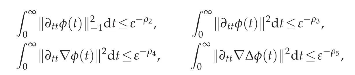
(3) φ(t)∈W1,2(0,∞;H3),or

Here ρj,j=1,2,3,4,5,6,7,8 are non-negative constants which depend on σ1,σ2,σ3.

We first carry out a coarse error estimate using a standard approach for time semi discretized schemes.

Proposition 3.1.(Coarse error estimate)Suppose that A,B are any non-negative number.Then for all N≥1,we have estimate

and

The index σ0+3 in(3.13)can be replaced with σ0if we take τ < ε1.5.

Proof.The following equations for the error function hold:

Pairing(3.14)with−∆−1adding(3.15)paired withwe get

where

For the right hand of(3.16),by using Cauchy-Schwartz inequality,we obtain the following estimate:

For J5of the right side of(3.16),by using δtten+1=δten+1−δten,we have

where

For the R1,...,R5terms,we have following estimates:

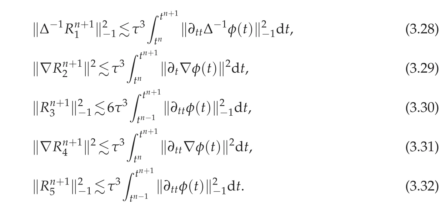
Substituting J1,···,J6into(3.16),we have

where

Taking η =ε/2,multiplying(3.33)by 2τ,we obtain(3.12)by using inequality ka+bk2≤2kak2+2kbk2and estimates(3.28)-(3.32).Then by summing(3.33)for n=1···N,we obtain

where

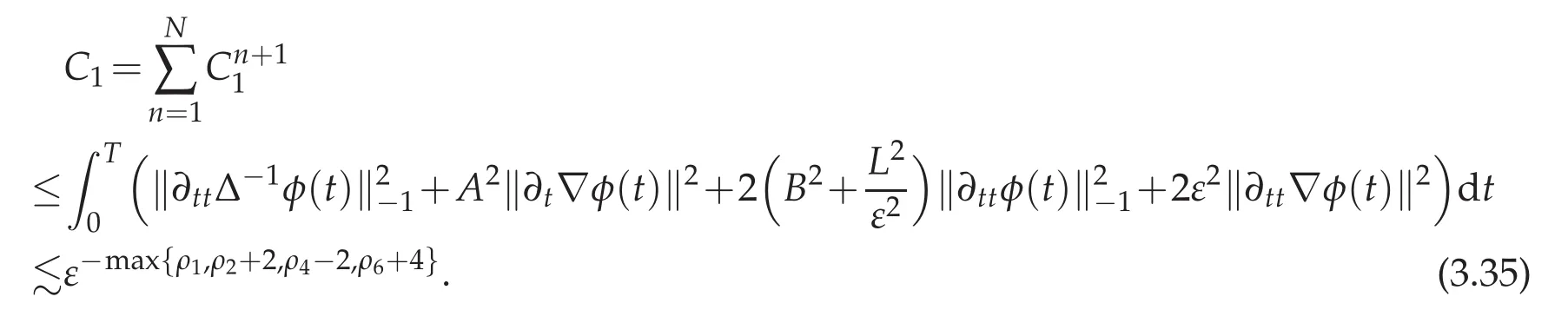
by discrete Gronwall inequality and assumption(3.9),we get(3.13).

Proposition3.1 is the usual error estimate,in which the error growth depends on T/ε3exponentially.To obtain a finer estimate on the error,we need to use a spectral estimate of the linearized Cahn-Hilliard operator by Chen[7]for the case when the interface is well developed in the initial condition.

Lemma 3.2.Let φ(t)be the exact solution of the Cahn-Hilliard equation(1.3)with interfaces are well developed in the initial condition(i.e.conditions(1.9)-(1.15)in[7]are satisfied).Then there exist 0<ε0≪1 and positive constant C0such that the principle eigenvalue of the linearized Cahn-Hilliard operatorsatisfies for all t∈[0,T]

for ε∈(0,ε0).

The following lemma shows the boundedness of the solution to the Cahn-Hilliard equation,provided that its sharp-interface limit Hele-Shaw problem has a global(in time)classical solution.This is a condition of the finer error estimate.

Lemma 3.3.Suppose that f satisfies Assumption 3.1,and the corresponding Hele-Shaw problem has a global(in time)classical solution.Then there exists a family of smooth initial functions{φε0}0<ε≤1and constants ε0∈(0,1]and C>0 such that for all ε∈(0,ε0)the solution φ(t)of the Cahn-Hilliard equation(1.3)with the above initial data φε0satisfies

Proof.See[20]and[1]for the detailed proof.

Now we present the refined error estimate.

Theorem 3.1.Suppose all of the Assumption 3.1,3.2,3.3 hold and B>L/2ε.Let time step τ satisfy the following constraint

then the solution of(2.3)-(2.4)satisfies the following error estimate

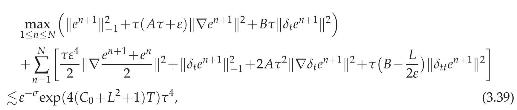
where σ=max{ρ1+4,ρ2+6,ρ4+2,ρ5−8,ρ6+8,ρ7−2,σ0}.

Proof.(i)To get a better convergence result,we re-estimate J5,J6in(3.16)as

For J8,by Taylor expansion,there exists ϑn+1betweensuch that

where C2=Here we assume that the conditions of Lemma 3.3 are satisfied.

Substituting J1,···,J8into(3.16),then we have

We need to bound the last three terms on the right hand side of above inequality.

(ii)To control theterm,we pair(3.14)withthen add(3.15)paired with−δten+1,to get

Analogously,applying the method for J1,···,J4toyields

Forof(3.45),we have

where ξn+1is a fixed number betweenNow,we estimate the first term on the right hand side of(3.50).

Combination of(3.50)and(3.51)yields

Substitutinginto(3.45),we have

Combining(3.44)and(3.53),then using triangle inequality(3.28)-(3.32)and following estimates

we obtain

where

(iii)We now estimate the last two terms of the right hand side of(3.59).The spectrum estimate(3.36)leads to

Applying(3.61)with a scaling factor(1−η1)close to but smaller than 1,we get

On the other hand,

Now,we estimate the L3term.By interpolating L3between L2and H1then using Poinc are inequality for the error function,we get

where K is a constant independent of ε and τ.We continue the estimate by using

to get

where Gn+1=

Now plugging equation(3.62),(3.63)and(3.64)into(3.59),we get

Take η1=ε3,η2=ε,η=ε4/11,˜η=ε−6,such that

Take

such that

Summing up(3.65),(3.66)and(3.68),we get

Now,if Gn+1is uniformly bounded by constant ε4/4,we can multiply by 2τ on both sides of inequality(3.69),and sum up for n=1 to N to get the following estimate

where

Choose τ ≤ 1/(2C0+2L2),then we can get a finer error estimate by discrete Gronwall inequality and the assumption of first step error(3.9)

We prove this by induction.Assuming that the above estimate holds for all first N time steps.Sincethen the coarse estimate(3.12)leads to

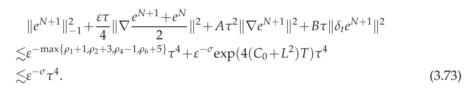
To obtain GN+1≤ε4/4,using(3.73),we easily get

Solving(3.74),we get

The proof is complete.

Remark 3.1.Note that the spectral estimate(3.36)is essential to the proof.Moreover,since the Crank-Nicolson discretization has no numerical diffusion,it is harder to bound the error growth than the BDF2 scheme.Here,we needto get the convergence,while in SL-BDF2 scheme,there is no such a requirement[38].

Remark 3.2.We used L∞bound assumption of the exact solution to handle the high order termoccured in(3.43).There is another way to control this term.By Cachy-Schwartz inequality,one only need to controlandThe L4term can be controlled by using Sobolev interpolation inequality as we did for theterm.The L2term of the error function can be controlled by aterm and

4 Numerical results

In this section,we numerically verify our schemes are energy stable and second order accurate in time.

We use the commonly used double-well potential F(φ)=(φ2−1)2.It is a common practice to modify F(φ)to have a quadratic growth rate for|φ|>1(since physically|φ|≤1),such that a global Lipschitz condition is satisfied[35],[9].To get a C4smooth double-well potential with quadratic growth,we introduce(φ)∈C∞(R)as a smooth mollification of

with a mollification parameter much smaller than 1,to replace F(φ).Note that the truncation points−2 and 2 used here are for convenience only.Other values outside of region[−1,1]can be used as well.For simplicity,we still denote the modified functionby F.

To test the numerical scheme,we solve(1.3)in tensor product 2-dimensional domainΩ =[−1,1]×[−1,1].We use a Legendre Galerkin method similar as in[36,42]for spatial discretization.Let Lk(x)denote the Legendre polynomial of degree k.We define

where ϕ0(x)=L0(x);ϕ1(x)=L1(x);ϕk(x)=Lk(x)−Lk+2(x),k=2,...,M−1,be the Galerkin approximation space for both φn+1and µn+1.Then the full discretized form for the SLCN scheme reads:

Findsuch that

This is a linear system with constant coefficients forwhich can be efficiently solved.We use a spectral transform with doubled quadrature points to eliminate the aliasing error and efficiently evaluate the integrationin equation(4.3).

We take ε=0.05 and M=63 and use two different initial values to test the stability and accuracy of the proposed schemes:

(1){φ0(xi,yj)}∈ R2M×2Mwith xi,yjare tensor product Legendre-Gauss quadrature points and φ0(xi,yj)is a uniformly distributed random number between −1 and 1(shown in the left picture of Figure 1);

(2)The solution of the Cahn-Hilliard equation at t=64ε3which takes φ0as its initial value(Denoted by φ1shown in the middle picture of Figure 1).

Figure 1:The two random initial values φ0, φ1and the state of φ1evolves 0.2 time unit according to the Cahn-Hilliard equation(1.3)with γ=1.

Table 1:The minimum values of A(resp B)(only values{0,2i,i=0,...,7}×γ are tested for A,only values{0,2i,i=0,...,7}are tested for B)to make scheme SL-CN stable when γ,B(resp A)and τ taking different values.

4.1 Stability results

Table 1 shows the required minimum values ofA(resp.B)with differentγ,B(resp.A)andτvalues for stably solving(not blow up in 4096 time steps)the Cahn-Hilliard equation(1.3)with initial valueφ0.The results for the initial valueφ1are similar.From this table,we observe that the SL-CN scheme is stable withA=0,B=0 whenτis small enough.If we takeA=0,thenB=16 will make the scheme unconditionally stable,the values ofγhas only a very small effect on the values ofB.But when we fixB,the caseγ=1 requires a much largerAvalue to make the scheme stable thanγ=0.0025 case,this is consistent to our analysis.

Figure 2 presents the discrete energy dissipation of the SL-CN scheme using several time step-sizes.We see clearly the energy decaying property is maintained.Moreover,astincreases,the differences betweenEandECNget smaller and smaller.

Figure 2:The discrete energy dissipation of the SL-CN scheme solving the Cahn-Hilliard equation with initial value φ1,and relaxation parameter γ =0.0025.Stability constant A=1,B=20 are used.

4.2 Accuracy results

We take initial valueφ1to test the accuracy of the two schemes.The Cahn-Hilliard equation withγ=0.0025 are solved fromt=0 toT=12.8.To calculate the numerical error,we use the numerical result generated usingτ=10−3as a reference of exact solution.The results are given in Table 2.We see that the scheme is second order accuracy inH−1,L2andH1norm.

Table 2:The convergence of the SL-CN scheme with B=40,A=0.1 for the Cahn-Hilliard equation with initial value φ1,parameter γ =0.0025.The errors are calculated at T=12.8.

5 Conclusions

We study the stability and convergence of a stabilized linear Crank-Nicolson scheme for the Cahn-Hilliard phase field equation.The scheme includes two second-order stabilization terms,which guarantee the unconditional energy dissipation theoretically.Use a standard error analysis procedure for parabolic equation,we get an error estimate with a prefactor depending on 1/ε exponentially.We then refine the result by using a spectrum estimate of the linearized Cahn-Hilliard operator and mathematical induction to get an optimal(second-order)convergence estimate in l∞(0,T;H−1)∩l2(0,T;H1)norm with a prefactor depends only on some lower degree polynomial of 1/ε.Numerical results are presented to verify the stability and accuracy of the scheme.

Acknowledgments

This work is partially supported by NSF of China No.11771439,No.11371358 and Major Program of under Grant NSF of China No.91530322.The authors thank Prof.Jie Shen and Prof.Xiaobing Feng for helpful discussions.

[1]Nicholas D.Alikakos,Peter W.Bates and X.Chen,Convergence of the Cahn-Hilliard equation to the Hele-Shaw model,Archive for Rational Mechanics and Analysis,128(2)(1994),165-205.

[2]S.M.Allen and J.W.Cahn,A microscopic theory for antiphase boundary motion and its application to antiphase domain coarsening,Acta Metall.Mater.,27(1979),1085-1095.

[3]J.Barrett,J.Blowey and H.Garcke,Finite element approximation of the Cahn-Hilliard equation with degenerate mobility,SIAM J.Numer.Anal.,37(1)(1999),286-318.

[4]B.Benesova,C.Melcher and E.Süli,An implicit midpoint spectral approximation of nonlocal Cahn–Hilliard equations,SIAM J.Numer.Anal.,52(3)(2014),1466-1496.

[5]A.Baskaran,P.Zhou,Z.Hu,C.Wang,S.Wise and J.Lowengrub,Energy stable and efficient finite-difference nonlinear multigrid schemes for the modified phase field crystal equation,J.Comput.Phys.,250(2013),270-292.

[6]John W.Cahn and John E.Hilliard,Free energy of a nonuniform system,I.interfacial free energy.J.Chem.Phys.,28(2)(1958),258-267.

[7]X.Chen,Spectrum for the Allen-Cahn,Cahn-Hillard,and phase- field equations for generic interfaces,Commun.Part.Diff.Eq.,19(7)(1994),1371-1395.

[8]Luis A.Caffarelli and Nora E.Muler,An L∞bound for solutions of the Cahn-Hilliard equation,Arch.Rational Mech.Anal.,133(2)(1995),129-144.

[9]N.Condette,Christ of Melcher and Endre Süli,Spectral approximation of pattern-forming nonlinear evolution equations with double-well potentials of quadratic growth,Math.Comp.,80(273)(2011),205-223.

[10]L.Q.Chen and J.Shen,Applications of semi-implicit Fourier-spectral method to phase field equations.,Comput.Phys.Commun.,108(2-3)(1998),147–1588.

[11]W.Chen,C.Wang,X.Wang and S.M.Wise,A linear iteration algorithm for a second order energy stable scheme for a thin film model without slope selection,J Sci.Comput.,59(3)(2014),574-601.

[12]Q.Du and R.A.Nicolaides,Numerical analysis of a continuum model of phase transition,SIAM J Numer.Anal.,28(5)(1991),1310-1322,.

[13]A.E.Diegel,C.Wang and S.M.Wise,Stability and convergence of a second order mixed finite element method for the Cahn-Hilliard equation,IMA J Numer.Anal.,36(4)(2016),1867-1897.

[14]C.Elliott and H.Garcke,On the Cahn-Hilliard Equation with Degenerate Mobility,SIAM J Math.Anal.,27(2)(1996),404–423.

[15]Charles M.Elliott and Stig Larsson,Error estimates with smooth and nonsmooth data for a finite element method for the Cahn-Hilliard equation,Math.Comp.,58(198)(1992),603-630,S33-S36.

[16]C.M.Elliott and A.M.Stuart,The global dynamics of discrete semilinear parabolic equations,SIAM J.Numer.Anal.,30(1993),1622-1663.

[17]D.J.Eyre,Unconditionally gradient stable time marching the Cahn-Hilliard equation,in Computational and Mathematical Models of Microstructural Evolution(San Francisco,CA,1998),Mater.Res.Soc.Sympos.Proc.,529(1998),39-46.

[18]X.Feng,Fully discrete finite element approximations of the Navier-Stokes–Cahn-Hilliard diffuse interface model for two-phase fluid flows,SIAM J.Numer.Anal.,44(3)(2006),1049-1072.

[19]X.Feng and A.Prohl,Error analysis of a mixed finite element method for the Cahn-Hilliard equation,Numer.Math.,99(1)(2004),47-84.

[20]X.Feng and A.Prohl,Numerical analysis of the Cahn-Hilliard equation and approximation of the Hele-Shaw problem,Interfaces Free Bound,7(1)(2005),1-2.

[21]X.Feng,T.Tang and J.Yang,Stabilized Crank-Nicolson/Adams-Bashforth schemes for phase field models.E.Asian J.Appl.Math.,3(1)(2013),59-80.

[22]D.Furihata,A stable and conservative finite difference scheme for the Cahn-Hlliard equation,Numer.Math.,87(4)(2001),675-699.

[23]F.Guilln-Gonzalez and G.Tierra,On linear schemes for a Cahn-Hilliard diffuse interface model,J.Comput.Phys.,234(2013),140-171.

[24]F.Guilln-Gonzalez and Giordano Tierra,Second order schemes and time-step adaptivity for Allen-Cahn and Cahn-Hilliard models,Comput.Math.Appl.,68(8)(2014),821-846.

[25]H.Gomez and T.J.R.Hughes,Provably unconditionally stable,second-order time-accurate,mixed variational methods for phase- field models,J.Comput.Phys.,230(13)(2011),5310-5327.

[26]J.Guo,C,Wang,S,M.Wise and X.Yue,An H2convergence of a second-order convex splitting, finite difference scheme for the three-dimensional Cahn-Hilliard equation,Commun.Math.Sci,14(2)(2016),489-515.

[27]D.Han,A.Brylev,X.Yang and Z.Tan,Numerical analysis of second order,fully discrete energy stable schemes for phase field models of two phase incompressible flows,J.Sci.Comput.,70(2017),965-989.

[28]Y.He,Y.Liu and T.Tang,On large time-stepping methods for the Cahn-Hilliard equation,Appl.Numer.Math.,57(5-7)(2007),616-628.

[29]J.Kim,K.Kangand J.Lowengrub,Conservative multigrid methods for Cahn-Hilliard fluids,J.Comput.Phys.,193(2)(2004),511-543.

[30]D.Kessler,R.H.Nochetto and A.Schmidt, A posteriori error control for the Allen-Cahn problem:circumventing Gronwall’s inequality,ESAIM:Math.Model.Numer.Anal.,38(01)(2004),129-142.

[31]D.Li and Z.Qiao,On second order semi-implicit Fourier spectral methods for 2d Cahn-Hilliard equations,J Sci.Comput.,70(1)(2017),301-341.

[32]D.Li,Z.Qiao and T.Tang,Characterizing the stabilization size for semi-implicit Fourierspectral method to phase field equations,SIAM J Numer.Anal.,54(3)(2016),1653-1681.

[33]C.Liu and J.Shen,A phase field model for the mixture of two incompressible fluids and its approximation by a Fourier-spectral method,Physica D,179(3-4)(2003),211-228.

[34]F.Magaletti,F.Picano,M.Chinappi,L.Marino and C.M.Casciola,The sharp-interface limit of the Cahn–Hilliard/Navier–Stokesmodel for binary fluids,J Fluid.Mech.,714(2013),95-1263.

[35]J.She nand X.Yang,Numerical approximations of Allen-Cahn and Cahn-Hilliard equations,Discrete Cont.Dyn.A,28(2010),1669-1691.

[36]J.Shen,X.Yang and H.Yu,Efficient energy stable numerical schemes for a phase field moving contact line model,J.Comput.Phys.,284(2015),617-6305.

[37]X.Wu,G.J.van Zwieten and K.G.van der Zee,Stabilized second-order convex splitting schemes for Cahn-Hilliard models with application to diffuse-interface tumor-growth models,Int.J.Numer.Meth.Biomed.Engng.,30(2)(2014),180-203.

[38]L.Wang and H.Yu,Two efficient second order stabilized semi-implicit schemes for the Cahn-Hilliard phase- field equation,arXiv:1708.09763,submitted to J.Sci.Comput.,August 2017.

[39]C.Xu and T.Tang,Stability analysis of large time-stepping methods for epitaxial growth models,SIAM J.Num.Anal.,44(2006),1759-1779.

[40]X.Yang,Linear, first and second-order,unconditionally energy stable numerical schemes for the phase field model of homopolymer blends,J.Comput.Phys.,327(2016),294-316.

[41]X.Yang and L.Ju,Efficient linear schemes with unconditional energy stability for the phase field elastic bending energy model,Comput.Method.Appl.Mech.Eng.,315(2017),691-712.

[42]X.Yang and H.Yu,Efficient second order energy stable schemes for a phase- field moving contact line model,arXiv:1703.01311,submitted to SIAM J.Sci.Comput.,2017.

[43]X.Yang,J.Zhao,Q.Wang and J.Shen,Numerical approximations for a three components Cahn-Hilliard phase- field model based on the invariant energy quadratization method,Math.Models Methods Appl.Sci.,27(2017),199.

[44]J.Zhu,L.-Q.Chen,J.Shen and V.Tikare,Coarsening kinetics from a variable-mobility Cahn-Hilliard equation:Application of a semi-implicit Fourier spectral method,Phys.Rev.E,60(4)(1999),3564-3572.

[45]Z.Zhang,Y.Ma and Z.Qiao,An adaptive time-stepping strategy for solving the phase field crystal model,J.Comput.Phys.,249(2013),204-215.