Spectral Element Methods for Stochastic Differential Equations with Additive Noise

Chao Zhang,Dongya Gu and Dongya Tao

School of Mathematics and Statistics,Jiangsu Normal University,Xuzhou 221116,P.R.China.

1 Introduction

Many problems in science and engineering can be characterized by differential equations.However,deterministic differential equations can not reveal the essence of these problems well due to the existence of accidental phenomena and small probability events. Therefore,many scholars consider stochastic differential equations to describe these problems,see[10,22,23]and etc,and the references therein.

Since the solution of a stochastic differential equation(SDE)is a stochastic process,it is difficult to reveal visually the information the process contains.Recently,there are many works to study the numerical solution for stochastic ordinary differential equations(SDEs).Euler-Maruyama method,Milstein method and Runge-Kutta method were proposed to solve SDEs numerically,see[3,4,13,16,17,19,20,31]and the references therein.

On the other hand,many authors investigated the numerical methods for stochastic partial differential equations(SPDEs).Allen et al.[1],Mcdonald[21],Gyöngy[14,15]used finite difference method to study the numerical solutions of linear SPDEs driven by additive white noise.Also,Walsh[28],Du and Zhang[11]studied finite element method for linear SPDEs driven by special noises.Moreover,Caoet al.[6,7,8],Theting[26,27],Yan[29]and etc,have also made some contributions.

As we know, spectral methods take orthogonal polynomials (such as Legendre, Chebyshev,Jacobi,Laguerre and Hermite polynomials)as the basis functions to approximate the solutions of problems in mathematical physics,and tend to have higher accuracy,see[5,12,25].Recently,some scholars are trying to study SPDEs by spectral methods.Shardlow[24]took the eigenvectors ofsubject to Dirichlet boundary condition as the basis functions and used spectral method to approximate the noise.Cao and Yin[9]studied spectral Galerkin method for stochastic wave equations driven by space-time white noise.In addition,Yin and Gan[30]proposed the Chebyshev spectral collocation method to solve a certain type of stochastic delay differential equations.

In the present work,we will try to solve stochastic equations by using spectral element methods.We begin with taking the SDEs driven by white noise into consideration.As we know,the regularity of the solutions of the original stochastic differential equations plays an important role in priori error estimates of the numerical solutions.Unfortunately,the regularity estimates are usually very weak because of the existence of white noise.In order to overcome this difficulty,we will approximate the white noise process by piecewise constant random process as in[1],and apply the Legendre spectral element method for the corresponding stochastic differential equation.We prove the numerical solution converges to the original solution.Moreover,the accuracy of the proposed scheme is indicated by the provided computational results.The other part is that we use spectral element methods to solve stochastic differential equations driven by colored noise numerically.Analogous to the way to deal with white noise,it is nature to use an finite dimensional noise to discretize the colored noise(see[11]),which could improve the regularity of the solutions of the original stochastic differential equations.Therefore,the relevant stochastic differential equation is capable of being approximated by the Legendre spectral element scheme.Furthermore,the numerical results show the high accuracy of spectral element methods.

This paper is organized as follows.In the next section,we study numerical solutions of stochastic differential equations driven by white noiseusing spectral element methods,and the error estimates as well as the numerical results are presented.In Section 3,we use spectral element methods to solve stochastic differential equations driven by colored noise numerically.The final section is for conclusion remarks.

2 Numerical solutions of SDEs driven by white noise

We consider the following stochastic problem driven by white noise

where(x)denotes white noise,g(x)is a deterministic function andbis a constant.

The integral form of(2.1)has the form

wherek(x,y)=x∧y−xyis Green’s function associated with the elliptic equation

Multiplying the equation(2.1)byφ(x)and integrating by parts onI,we derive that a weak formulation of(2.1)is

whereφ∈C2(0,1)∩C0[0,1].

Remark 2.1.Buckdahn and Pardoux[2]proved existence and uniqueness of solutions to(2.2)and(2.3).Meanwhile,(2.2)and(2.3)are equivalent.

2.1 Approximation of white noise

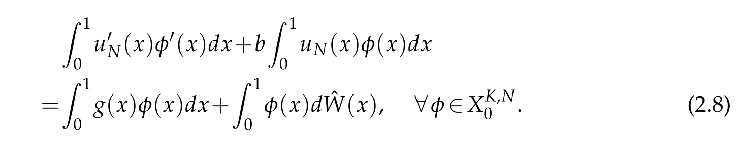
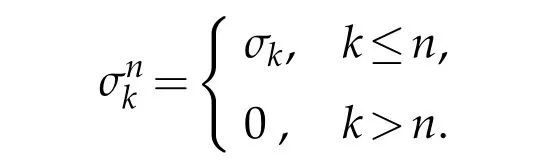
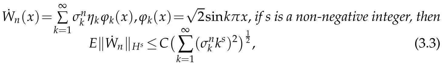
Partition the intervalIinto 0=x0

where

η1,η2,···,ηKare a sequence of random variables that are independent and identically distributed(i.i.d.)and subject to the standard normal distributionN(0,1),

Substitutingd(y)fordW(y)in(2.2),we can get

According to Theorem 2.2 in[1],we have the following regularity result.

Lemma 2.1.Letbe the solution of(2.5)with g∈L2(0,1)and b≥0.Then∈H2(0,1)∩(0,1)withwhere constant C depends only on g.

From Theorem 2.1 in[1],we have the estimation between u and.

Lemma 2.2.Letbe the solution of(2.5),and u be the solution of(2.2).There holds

where λ2=(x,y)dxdy<1.

Remark 2.2.Lemma 2.2 implies that if the mesh is sufficiently fine,then(x)is a good approximation to u(x),and(x)is smoother than u(x).

2.2 Spectral element methods for stochastic differential problem(2.1)

Denote(I)={u|u,u′∈L2(I),u(0)=u(1)=0},we substitute(x)for W(x),then the weak form(2.3)of the problem(2.1)can be written as

Let

where PNbe the space of the algebraic polynomials with degree at most N.Then the corresponding Galerkin scheme of(2.7)is to findsuch that

Define the Sobolev space:

By using Theorem 3.39 in[25],we obtain the following result on I directly.

Lemma 2.3.Ifthen for 1≤m≤N+1 andµ=0,1,

where C is a positive constant independent of,h,m and N.

Remark 2.3.In particular,for m=2,letand uNbe the solutions of(2.7)and(2.8),we have

Therefore,by the triangle inequality,Lemma 2.2,(2.9)and Lemma 2.1,successively,we have the following error estimates.

Theorem 2.1.Let u and uNbe the solutions of(2.1)and(2.8),respectively.Then we have

where C is a positive constant independent of h and N.

2.3 Numerical results

Let

Here,Lm(ξ)is the Legendre polynomial on(−1,1)with degree m,which satisfy that Lm(±1)=(±1)m,and fulfill the following relations.

In actual computation,we introduce the boundary-inner decomposition basis

We expand them into global variable by

where mi(ξ)=xi−1φ0(ξ)+xiφN(ξ),i=1,···,K,m=1,···,N−1.For ensuring the continuity of the solution of the problem,we must propose the basis functions at interfaces.Therefore,we introduce

where i=1,···,K−1.At the left and right endpoints,we define

So the global basis set are

Then,we expand the numerical solution of the problem(2.1)as follows:

Substituting the above expression into Galerkin scheme(2.8)and taking φ=ψl(x),l=0,···,KN,which yields that

Let us denote

Then the linear algebraic system(2.19)becomes the following compact form

To compute the errorEku−uNkL2,we set the state of random numbers to be 400,perform 10000 runs with different samples of noise for each computation,then for each sample calculateku−uNkL2,and finally,obtain the average value of ku−uNkL2.

For the problem(2.1)withb=,we take the test functionu(x)=x(1−x)sin3x.In Table 1,the values of the errorEku−uNkL2with variousNandKare listed.We can see that the errors decay asNandKincrease.Comparison with the numerical results in[1],Allen,Novosel and Zhang tookh=0.0294 and the smoother test functionu(x)=x(1−x),the accuracy of errors can only be reached toO(10−4).While in Table 1,though the test functionu(x)=x(1−x)sin3xis oscillatory,the accuracy can be reached toO(10−6)withN=8.This indicates that our new approach seems to be more accurate.

Table 1:The values of EkuN−ukL2.

3 Numerical solutions of SDEs driven by colored noise

Due to the existence of white noise,the solution to(2.1)has low regularity,thus it doesn’t achieve higher precision,which can be seen from Table 1.In this section,we will study numerical methods for stochastic differential equations driven by colored noise.

3.1 Properties of colored noise

LetW={W(t),t≥0}be a standard Wiener process and for fixedh>0,we define colored noise by(see[18])

This is a wide-sense stationary Gaussian process with zero means and with covariances

it thus has spectral density

In general,we may use the following abstract formulation to simulate colored noise(see[11]):

where the i.i.d.random sequence ηk∼N(0,1),the deterministic functions{ϕk(x)}form an orthogonal basis of L2(I)or its subspace,and the coefficients{σk}are to be chosen to ascertain the convergence of the series in the mean square sense with respect to some suitable norms.

Letapproachas n→∞in some appropriate sense,then an approximation of

where

As was shown by Du and Zhang[11],the faster the coefficients σkdecay,the smoother the noise trajectory˙Wn(x)looks.On the other hand,if the coefficients decay sufficiently slowly,then the trajectory can clearly resemble that of a white noise away from the boundary.In the end of this section,we will give the numerical results to demonstrate that different forms of coefficientsinduce different rates of convergence.

From Lemma 3.1 in[11],a bound is stated on˙Wnin the following lemma.

Lemma 3.1.For

provided that the right-hand side is convergent.

3.2 Spectral element methods for SDEs driven by colored noise

We consider the following stochastic problem driven by colored noise

where(x)denotes colored noise,g(x)is a deterministic function and b is a constant.

The integral form of the problem(3.4)is

and the weak form is

We replace dW(y)with dWn(y)in(3.5),and obtain

According to Theorem 3.1 in[11],the following lemma holds.

Lemma 3.2.Forif u andare the solutions of(3.5)and(3.7),respectively,then,for some constant C>0,

where λ2=b2k2(x,y)dxdy<1,(σ1,σ2,···,σk,···)t,

Substituting Wn(x)for W(x)in(3.6),the weak form(3.6)can be written as

and the corresponding Galerkin scheme of(3.4)is to findsuch that

Following the same line of Theorem 2.1,together with the triangle inequality,Lemma 3.2 and Lemma 2.3,we then have the following error estimates.

Theorem 3.1.Let u and uNare the solutions of(3.4)and(3.10),respectively.Then we have

where C is a positive constant independent of u,h,m and N.Furthermore,according to Lemma 3.1,for 2≤m≤N+1,we have

3.3 Numerical results

In actual computation,we expand the numerical solution of the problem(3.4)as follows:

whereare defined in(2.14)-(2.17).Substituting the above expansion in to Galerkin scheme(3.10)and takingφ=ψl(x),l=0,···,KN,we can obtain the following system of linear algebraic equations

Let us denote

Then we can rewrite the linear algebraic system(3.13)as

where the matrixS,Mis defined as in(2.20).

For numerical experiment,we letb=,and the test functionud(x)=x(1−x)sin3x.Then the exact solution to(3.4)is given byu(x)=ud(x)+us(x),where

The state of random numbers is also set to be 400.Tables 2-3 list the values of the errorEku−uNkL2withσk=respectively.The results indicate that the errors decay rapidly asNandKincrease.At the same time,they demonstrate that if the coefficientsσkdecay sufficiently fast,the numerical solution would be smoother.

Also,in[11],Du and Zhang tookand the smoother test functionud(x)=x(1−x),the accuracy of error estimates could only be reached toO(10−6)whenσk=While for spectral element methods,from Table 2,the accuracy of error estimates can be reached toO(10−13)withN=240,even if we take the oscillatory function asud(x)=x(1−x)sin3x.Forσk=took the samehand test function,Du and Zhang[11]get the accuracy of estimates reached toO(10−10).As we can see from Table 3,the accuracy can be reached toO(10−14)only withN=140.This demonstrates the accuracy of the proposed method.

Table 2:The values of EkuN−ukL2with σk=

Table 2:The values of EkuN−ukL2with σk=

K=1 K=2 K=3 N=20 3.97e−05 2.10e−05 1.41e−05 N=60 1.33e−05 6.71e−06 4.35e−06 N=100 7.91e−06 3.73e−06 2.37e−06 N=140 5.61e−06 2.56e−06 2.62e−09 N=180 4.26e−06 1.62e−06 1.48e−10 N=220 3.39e−06 9.54e−10 2.21e−11 N=240 2.83e−06 2.02e−10 2.32e−13

Table 3:The values of EkuN−ukL2with σk=

Table 3:The values of EkuN−ukL2with σk=

K=1 K=2 K=3 N=20 4.95e−08 6.13e−09 1.82e−09 N=60 1.87e−09 2.27e−10 6.71e−11 N=100 4.08e−10 4.87e−11 1.44e−11 N=140 1.50e−10 1.77e−11 1.12e−14

4 Conclusion

In this paper,the Legendre spectral element schemes were proposed for stochastic differential equations driven by white noise and colored noise,respectively.For stochastic differential equations driven by white noise,we improved the regularity of the solution by employing piecewise constant random process to approximate white noise process.Thus,the Legendre spectral element scheme was able to apply to approximate the corresponding stochastic differential equation.The error analysis was provided and the accuracy of the proposed scheme was showed by the numerical experiments.As for stochastic differential equations driven by colored noise,we approximated colored noise process by a finite dimensional noise and employed the Legendre spectral element scheme to the corresponding stochastic differential equation.The error estimation was presented and the numerical results demonstrated the high accuracy of the proposed schemes.

Although the spectral element methods was only considered for second order elliptic stochastic differential equations in the present work,it is suitable to other types of stochastic differential equations.

Acknowledgments

This work is supported in part by NSF of China No.11571151 and No.11771299,and Priority Academic Program Development of Jiangsu Higher Education Institutions.

[1]E.J.Allen,S.J.Novosel and Z.M.Zhang,Finite element and difference approximation of some linear stochastic partial differential equations,Stochastics Stochastics Rep.,64(1-2)(1998),117-142.

[2]R.Buckdahn and E.Pardoux,Monotonicity methods for white noise driven quasi-linear SPDEs,Diffusion Processes and related Problems in Analysis.,Vol.ı,1990.

[3]K.Burrage and P.M.Burrage,High strong order explicit Runge-Kutta methods for stochastic ordinary differential equations,Appl.Numer.Math.,22(1996),81-101.

[4]K.Burrage,P.M.Burrage and T.Tian,Numerical methods for strong solutions of stochastic differential equations:An overview,Proc.R.Soc.A:Math.Phys.Eng.Sci.,460(2004),373-402.

[5]C.Canuto,M.Y.Hussaini,A.Quarteroni and T.A.Zang,Spectral methods:evolution to complex geometries and applications to fluid dynamics,Springer-Verlag,Berlin,2007.

[6]Y.Cao,Finite element and discontinuous Galerkin method for stochastic helmholtz equation in two-and-three dimensions,J.Comput.Math.,26(5)(2008),702-715.

[7]Y.Cao,Z.Chen and M.Gunzburger,Error analysis of finite element approximations of the stochastic Stokes equations,Adv.Comput.Math.,33(2)(2010),215-230.

[8]Y.Cao,H.T.Yang and L.Yan,Finite element methods for semiline arelliptic stochastic partial differential equations,Numer.Math.,106(2007),181-198.

[9]Y.Cao and L.Yin,Spectral Galerkin method for stochastic wave equations driven by spacetime white noise,Commun.Pure Appl.Anal.,6(3)(2007),607-617.

[10]E.Cinlae,Introduction to stochastic processes,Englewood cliffs,New Jersey:Prentice-hall,Inc.,1975.

[11]Q.Du and T.Zhang,Numerical approximation of some linear stochastic partial differential equations driven by special additive noise,SIAM.J.Numer.Anal.,40(2002),1421-1445.

[12]B.Y.Guo,Spectral methods and their applications,World Scientific Publishing Co.Inc.,River Edge,NJ,1998.

[13]Q.Guo,W.Liu,X.Mao and R.Yue,The truncated milstein method for stochastic differential equations,arXiv:1704.04135v2.,2017.

[14]I.Gyöngy,Lattice approximations for stochastic quasi-linear parabolic partial differential equations driven by space-time white noise,I,Potential Anal.,9(1998),1-25.

[15]I.Gyöngy,Lattice approximations for stochastic quasi-linear parabolic partial differential equations driven by space-time white noise,II,Potential Anal.,11(1999),1-37.

[16]D.J.Higham,X.Mao and A.M.Stuart,Strong convergence of Euler-like methods for nonlinear stochastic differential equations,SIAM J.Numer.Anal.,40(2002),1041-1063.

[17]D.J.Higham,X.Mao and A.M.Stuart,Exponential mean square stability of numerical solutions to stochastic differential equations,London Mathematical Society J.Comput.Math.,6(2003),297-313.

[18]P.E.Kloedn and E.Platen,Numerical solution of stochastic differential equations,Springer-Verlag Berlin Heidelberg.,1999.

[19]X.Mao,The truncated Euler-Maruyama method for stochastic differential equations,J.Comput.Appl.Math.,290(2015),370-384.

[20]N.Mariko and N.Syoiti,A new high-order weak approximation scheme for stochastic differential equations and the Runge-Kutta method,Finance Stoch.,13(2009),415-443.

[21]S.Mcdonald,Finite difference approximation for linear stochastic partial differential equations with method of lines,Munich Personal RePEc Archive,2006.

[22]B.Øksendal,Stochastic differential equations.Springer-Verlag Berlin Heidelberg,2005.

[23]L.R.Rabiner,A tutorial on hidden Markov models and selected applications in speech secognition,Proceedings of IEEE.,77(2)(1989),257-286.

[24]T.Shardlow,Numerical methods for stochastic parabolic PDEs.Numer.Funct.Anal.Optim.,20(1999),121-145.

[25]J.Shen,T.Tang and L.L.Wang,Spectral methods:algorithms,analysis and applications,volume 41 of Series in Computational Mathematics.Springer-Verlag,Berlin,Heidelberg.,2011.

[26]T.G.Theting,Solving Wick-stochastic boundary value problems using a finite element method.Stochastics Stochastics Rep.,70(3-4)(2000),241-270.

[27]T.G.Theting,Solving parabolic Wick-stochastic boundary value problems using a finite element method,Stochastics Stochastics Rep.,75(1-2)(2003),49-77.

[28]J.B.Walsh,Finite element methods for parabolic stochastic PDES,Poten.Anal.,23(2005),1-43.

[29]Y.Yan,Semidiscrete Galerkin approximation for a linear stochastic parabolic partial differential equation driven by an additive noise,BIT.Numer.Math.,4(2004),829-847.

[30]Z.W.Yin and S.Q.Gan,Chebyshev spectral collocation method for stochastic delay differential equations,Adv.Difference Equ.,1(2015),1-12.

[31]R.Zeghdane,L.Abbaoui and A.Tocino.,Higher-order semi-implicit Taylor schemes for Itö stochastic differential equations,J.Comput.Appl.Math.,236(2011),1009-1023.