
Aerodynamics analysis of a hypersonic electromagnetic gun launched projectile
2020-07-02 03:16JinShenShoFnxinJiQingyuZhuJiDun
Defence Technology 2020年4期
Jin Shen , Sho-o Fn , Y-xin Ji , Qing-yu Zhu , Ji Dun
a College of Mechatronics Engineering, North University of China, No. 3, Xue Yuan Road, Tai Yuan, 030051, China
b Northwest Industries Group CO., Ltd., No.123, Xing Fu Middle Road, Xi’an, 710043, China
c Jilin Jiangji Special Industries CO., Ltd., No.17, Zun Yi West Road, Ji Lin,132021, China
d AVIC China Aero-Polytechnology Establishment, No. 7, Jing Shun Road, Beijing,100028, China
Keywords:Electromagnetic gun launched projectile Hypersonic aerodynamics Airframe configuration optimization Static margin Pendulum
ABSTRACT A hypersonic aerodynamics analysis of an electromagnetic gun (EM gun) launched projectile configuration is undertaken in order to ameliorate the basic aerodynamic characteristics in comparison with the regular projectile layout. Static margin and pendulum motion analysis models have been applied to evaluate the flight stability of a new airframe configuration. With a steady state computational fluid dynamics (CFD) simulation, the basic density, pressure and velocity contours of the EM gun projectile flow field at Mach number 5.0, 6.0 and 7.0 (angle of attack = 0°) have been analyzed. Furthermore, the static margin values are enhanced dramatically for the EM gun projectile with configuration optimization. Drag, lift and pitch property variations are all illustrated with the changes of Mach number and angle of attack.A particle ballistic calculation was completed for the pendulum analysis.The results show that the configuration optimized projectile,launched from the EM gun at Mach number 5.0 to 7.0,acts in a much more stable way than the projectiles with regular aerodynamic layout.
1. Introduction
According to the 21st Century United States(US)Navy Operation Concept,an electromagnetic gun would be fielded to strike harder in future maritime disputes. Different to traditional artillery, projectiles obtain a higher speed, efficiency and longer range when launched from an EM gun[1].On May 10th,2017,General Atomics’Blitzer railgun system successfully launched a hypersonic projectile with over 30,000 gees accelerations at the US Army Dugway Proving Ground in Utah [2]. This meant that projectiles needed to be stable and reliable under harsh launching conditions in an EM gun.For large caliber projectiles,such as 155-mm Compatible hyper velocity projectile (HVP), there fins were installed at the tail in order to keep the ammunition in stable flight [3]. For small diameter projectiles,they behave well when spinning at a high rate.For a propellant powered rifle, the rifling gripped the projectile by the jacket and forced it to spin at a high rate as it was pushed down the bore [4]. If launched from an EM railgun, there is no rifles to spin the projectile keep it aerodynamically stable.Furthermore,limits of caliber and processing technology make fin installation outside of the cylinder part impossible for projectiles. As a result, finding a way to make the EM gun fire projectiles with fin-stability was significant.Defense Advanced Research Projects Agency (DARPA)’s Extreme Accuracy Tasked Ordnance (EXACTO)program developed a self-steering smart bullet which had its own fixed tail fins for keeping its trajectory steady (Fig. 1). Differing from the original bullet configuration, a counterweight near the nose pushed the smart bullet’s center of gravity (CG) ahead of its center of aerodynamic pressure (CP) [5]. A smart bullet had been tested in a 12.7 mm smooth bore gun with an initial velocity under Mach number 3.0.The stability of smart bullet had been verified.It shows that this kind of projectile configuration is better for maintaining flight stability [6].
The smart bullet’s aerodynamic configuration was desirable for EM gun projectile design. This paper was mainly focused on the aerodynamics of an EM gun launched projectile with special aerodynamic layout.
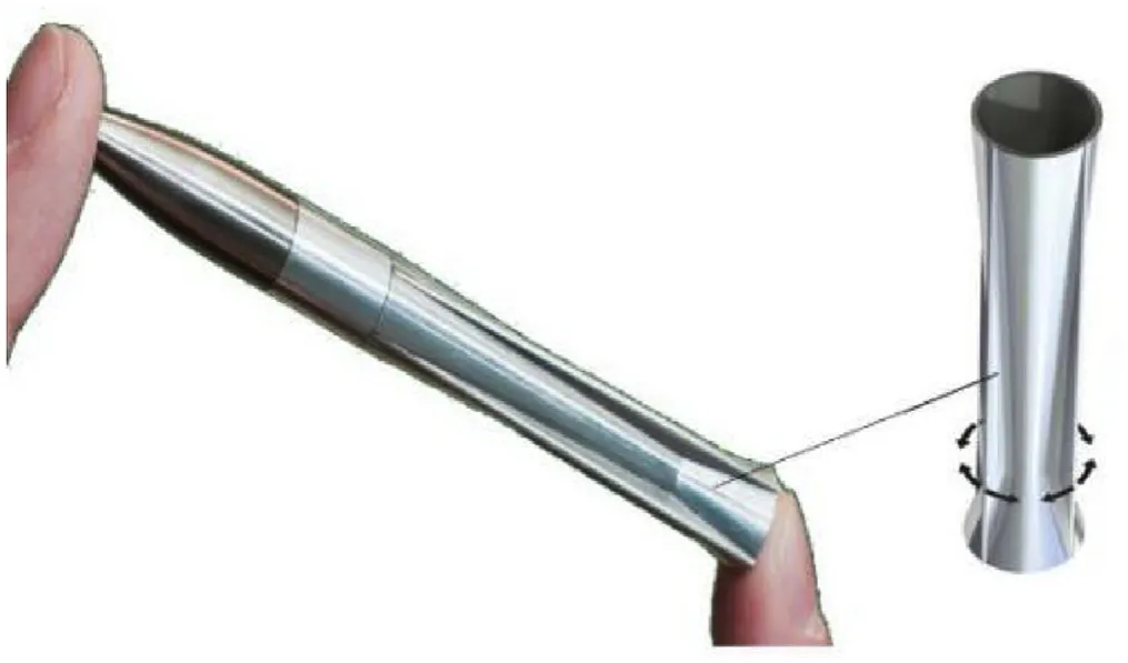
Fig.1. Smart projectile.
Understanding the aerodynamics of projectiles was critical for the designing of stable configurations and contributed significantly to the overall performance of weapon systems[7,8].As a result,the prediction of projectile stability was very important,particularly for an EM gun launched projectile in hypersonic flight.
E.Y.Fournier et al.[9]investigated the aerodynamic coefficients,base pressure surveys, base flow visualization, and shock patterns of a hypersonic cone-cylinder-flare projectile by CFD means. By comparing with free flight experimental results, it demonstrated the absence of a relation between the aerodynamic coefficients and the projectile configuration. David D. Young et al. [10] completed laminar and turbulent computations of a segmented projectile in order to study unsteady hypersonic aerodynamics.As discussed by S.D. Naik [11], a stability criterion for a subscribed projectile was provided which was based on Lyapunov’s second method. Paul Weinacht[12]used a viscous CFD approach in order to predict the aerodynamic performance of projectiles in supersonic flight. This represented the capability for predicting the linear aerodynamics for the high-speed, low angle of attack flight of aerodynamically smooth axisymmetric projectiles. Jubaraj Sahu [13] computed the unsteady aerodynamics which are associated with the free flight of the finned projectile at supersonic speeds by CFD which contained an advanced time-accurate Navier-Stokes technique.The computed results were then compared with the free flight tests data. For the researches about numerical simulation of hypersonic fluidstructure interaction, Prakash et al. [14] presented a fifth-order shock-fitting method for numerical simulation of thermal and chemical nonequilibrium in hypersonic flows.The new method has been tested and validated for a number of test cases over a wide span of free stream conditions. Jack and Peretz [15] reviewed the area of the aeroelastic and aerothermoelastic analysis in hypersonic flow.The authors stated the modeling approaches vary from simple approximate theories to high-fidelity numerical approaches. For example, computational fluid dynamics (CFD) and computational thermostructural dynamics (CTSD). And they introduced some computationally efficient researches of hypersonic aerothermoelastic modeling method. Brian and Joseph [16] evaluated existing gaps in computational fluid dynamics (CFD) technology with an emphasis on hypersonic flow modeling. They also compared DPLR,VULCAN,CFD++and FLUENT which were used in hypersonic vehicle analysis. Wang et al. [17] illustrated a twodimensional immersed boundary method for fluid-structure interaction with compressible multiphase flows involving large structure deformations.The results agreed well with the published data and experiment. And they demonstrate the versatility of this method by applying it to a flexible plate interacting with multiphase flows.
In this paper, a system was built to efficiently generate an aerodynamic stability analysis procedure for an EM gun launched projectile in atmospheric flight. Based on projectile aerodynamic theory, a stability criterion had to be established. With CFD simulations at different Mach numbers and angles of attack, the basic EM gun projectile aerodynamic properties were compared with regular projectile configuration. In addition, the projectile pendulum motion characteristics were analyzed based on particle ballistic simulation results.
2. Methods
The EM gun launched projectile is designed with a fin-stabilized configuration and it assumes that the projectile is not spinning.It is stated that statically stable finned projectiles without spinning are always dynamically stable [18].
2.1. The static margin
The static margin of a projectile is the precondition of its stabilization flight[19].If a fin-stabilized projectile is statically stable,CP is behind CG,as shown in Fig.2.Thus,a stabilizing moment,Mz,acts on the projectile to reduce the pendulum angle δ and keeps it more stable.
The static margin is a relative criterion of the CP-CG separation.The static margin B is written as follows:
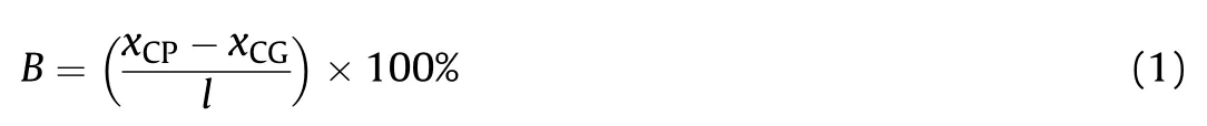
If there is a stable moment which acts on CG,B should be greater than zero.Ordinarily,a fin-stabilized projectile,with a static margin of greater than 10%,will maintain a steady state during flight in the air [20].
2.2. Pendulum motion
If there is no nutation in the flight of a fin-stabilized projectile,the stabilizing moment will gradually reduce the pendulum angle.Due to inertia, the projectile acts a pendulum motion around the CG. The stabilizing moment prevents projectiles from overturning but not the pendulum. The equatorial damping moment, accomplished during the projectile’s flight, will dampen pendulum movement and decrease pendulum frequency gradually[21].
Without taking ballistic curvature into account, the swinging angle of attack of the projectile is shown in Eq. (2).
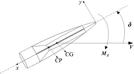
Fig. 2. The relative position of CG and CP for a fin-stabilized projectile.

It can be demonstrated by,
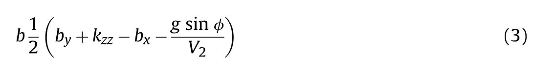
where bx, by, kzand kzzare related to the projectile aerodynamic,these parameters can be shown as,
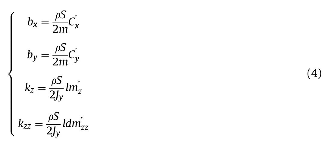

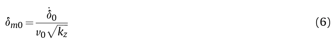
where C’x, C’y, m’zand m’zzare functions of the projectile’s configuration and Mach number[22].Eq.(2)can also be determined from,According to Eq.(5),δ acts a periodical change with time.If b is less than zero, the pendulum motion will be attenuated. The characteristic quantities of the pendulum are shown as follows:
1. Greatest amplitude
2. Pendulum period
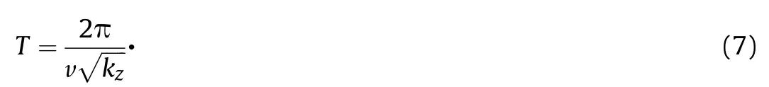
Substituting Eq. (4) into Eq. (7),
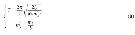
3. Pendulum wavelength
The wavelength is the flight distance for once pendulum movement. It can be shown by,
The stabilizing moment is illustrated as,

Eq. (10) is also demonstrated by Ref. [22],
Based on Eqs. (10) and (11), there is a relational expression shown as,

And the pendulum wavelength is also represented by,
In order to maintain the projectile’s stability, the pendulum wavelength λ and angle δ should be controlled within limits.
3. Numerical approach
Computational fluid dynamic(CFD)calculations were routinely used in order to accurately predict the static aerodynamic coefficients (e.g. drag, longitudinal, and lateral forces and moments)and flow phenomena of many geometrically complex projectiles and missiles [23].
3.1. Geometry
The difference between a smart projectile(Fig.1)and an EM gun launched projectile was that fins were installed on the curved portion because of the caliber limit(less than 12.7 mm).The short cylindrical body connects the armature in an EM gun bore.An EM gun launched projectile with a special aerodynamic layout was compared to the regular projectile configuration in Fig. 3. There were four slots in the circumferential direction of the EM gun projectile. The structure sketch is shown in Fig. 4.
In the above sketch,the length of projectile l was consist of the nose length ln, the slot length ls(equals to ls1plus ls2) and the cylinder length lc. Because the strength consideration of the projectile body,lswas 40 mm,lnand lcwere 10 mm,respectively.The ratio of ls1and ls2was 3:1.The diameter of φ was 5 mm.The model’s slot angle θ is 90°.
3.2. Mesh
The computational domains for the EM gun projectile consisted of 3.1 million cell structured hexahedral grids which were generated using ANSYS® ICEM CFDTM 16.0 Windows 64-bit and both were exported in double precision format(see Figs.5 and 6).Using a ‘top-down’ grid generation, an ‘O-grid’ technique was used to simulate the projectile and fin configuration[24].The far field was located 100 mm upstream of the nose and 200 mm downstream of the base.The grid diameter to the far field boundary was 20 times the projectile in the axial direction. A boundary layer spacing of 0.0005 mm was utilized for all Mach number regimes.
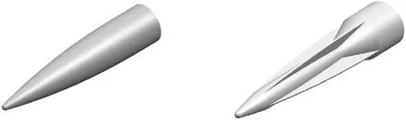
Fig. 3. Comparison of the regular projectile configuration(left) and EM gun projectile(right) shape.
Fig. 4. Sketch of the EM gun projectile structure.
Fig.5. Sketch of the structured mesh.a).full grid view of symmetry plane,b).close-up of grid near projectile.
Fig. 6. Grid on symmetry plane.
3.3. Navier-Stokes CFD
ANSYS Fluent, commercial version 16.0, was used during the computation.A density-based method was chosen in order to solve the compressible flow. In this solver, a second-order upwind, implicit, Roe-FDS system was utilized in order to capture the shockwave much easier in hypersonic air flow and improved the convergence and stability in computation[25].A far field boundary was used for EM gun projectile aerodynamic simulations which produced a set of free-stream Mach numbers and static parameters.
Multiple turbulence models were used for the steady-state computation - Spalart-Allmaras model, Standard k-ε model,Standard and SST k-ω model [26]. During the hypersonic flow, the turbulence boundary layer interacted with the shockwave, which induced boundary layer separation. The Spalart-Allmaras model which solves directly a transport equation for the eddy viscosity,became quite popular because of its reasonable results for a wide range of flow problems and its numerical properties [27]. Paciorri et al. [28] used The Spalart-Allmaras turbulence model in a cellcentered finite volume solver and tested for several hypersonic flow configurations. The results shown an excellent agreement with the experimental data. U. Goldberg [29] tested the performance of the Spalart-Allmaras model in predicting hypersonic flow heat transfer. The Spalart-Allmaras model nevertheless predicted the heat transfer distribution quite well according to the results.Roy and Blottner [30] studied hypersonic transitional flows over a flat plate and a sharp cone by using different turbulence models including the Spalart-Allmaras model.The Spalart-Allmaras model performs the best with regards to model sensitivity and model accuracy.
According to the references,a Spalart-Allmaras model provided a better simulation in the boundary layer and it was ideal for solving the flow wall confinement problems. With significant engineering verification, a Spalart-Allmaras model has been applied in the aeronautics and aerospace fields [31,32]. In this paper, the Spalart-Allmaras model was adopted as turbulence model in Section 4.
The following simulations were completed using a dual-core 2.50 GHz Intel(R) Core(TM) i5-7200U CPU, 12 logical processors,DELL work-station.It took 2-5 s of CPU time per iteration and there was a minimum of 5000 iterations for every computation case.
4. Results and discussion
4.1. Flow visualization
This section displays the visualization of the model static simulations. During the static simulations, there were minor differences between the different Mach number cases. Fig. 7 demonstrates density contours of EM gun projectile flow field at Mach numbers 5.0,6.0,7.0 and a zero-degree angle of attack.These figures show that there was an obvious swept bow which occurred at the nose. In addition, the same phenomenon occurred at joints between fins and the cylinder part of the projectile. As the Mach number increased, the angle of shock wave at the nose decreased.This means that shock approaches the airframe much closer as the Mach number increases. In addition, the density at the projectile bottom reduces significantly.
Fig.7. Density contours of different computation cases of zero angle of attack:a).Mach number 5.0; b). Mach number 6.0; c). Mach number 7.0.
Fig. 8 illustrates the airframe exterior pressure distributions at different Mach numbers. During hypersonic flow, the maximum pressures on the projectile nose are 1.87 × 10⁵, 2.98 × 10⁵and 4×10⁵Pa at Mach numbers 5.0,6.0 and 7.0.Around the nose,there are circular cone areas of high pressure which appeared. In addition, fields of relatively high-pressure arose among the four fins near the cylinder.
Fig. 9 represents an outline of typical static steady state flow fields for the EM gun projectile at a zero angle of attack. Velocity contours are shown on the symmetry plane at representative free stream of Mach number 5.0, 6.0 and 7.0, respectively. Typical flow features are observed,low speed flows at the base of the projectiles.
4.2. Static margin simulations
Fig. 8. Pressure contours of different computation cases of zero angle of attack: a).Mach number 5.0; b). Mach number 6.0; c). Mach number 7.0.
In this part, steady-state simulations were completed at Mach numbers 5.0, 6.0 and 7.0 with angles of attack of 0°, 2°, 4°and 6°.The projectile was assumed to be without rolling.Fig.10 shows the changes of CP axial position which are associated with the Mach number. This illustrates the axial position of CP approach to the base of the projectile as the Mach number increases. As shown by the curves,the increase in the ratio of value for regular projectiles is larger than for EM gun ones.From measuring of the 3D model,the axial positions of CG are 38.98 mm for the regular model and 42.33 for the EM gun projectile. For the regular model, there is just one case(Mach number 7.0)in which CP is between CG and the bottom of the airframe. A projectile with a regular configuration cannot maintain a relatively stable flight state at Mach numbers 5.0 and 6.0. However, as shown in Fig.10, the EM gun projectile axial positions of the CP are all greater than the CG which means that the projectile with optimized aerodynamic layout flew more steadily than the regular one.
According to Table 1,the static margins are all greater than 10%for EM gun projectiles. However, the regular cases are below the static margin 10% criterion from Mach number 5.0 to 7.0. This proves that the static margin is significantly affected by the optimization of EM gun projectile configuration.To put it simply,flight stability will be improved if the regular airframe configuration is optimized to what is shown in Fig. 3.
Fig. 9. Velocity contours of different computation cases of zero angle of attack: a).Mach number 5.0; b). Mach number 6.0; c). Mach number 7.0.
Fig.10. Axial positions comparison of CP between regular and EM gun projectile.
Table 1 Comparison of the static margin.
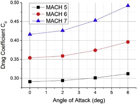
Fig.11. Drag coefficients vs. angle of attack.
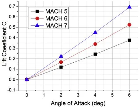
Fig.12. The comparison of lift coefficients with different Mach number and angle of attack.
The drag coefficient, lift coefficient and pitch moment coefficient changes, varied according to Mach number and angle of attack,and are shown in Figs.11,12 and 13.In Fig.11,the value of Cdincreases slowly at the same Mach number as the angle of attack increases.Additionally,at the same angle of attack,Cdalso increases slowly from Mach number 5.0 to 7.0.In Fig.12,the lift coefficient,Cl,acts a same changing tendency with Cd.Obviously,the values of Clare all zero at an angle of attack of 0°.Clis directly proportionate to Mach number and angle of attack. With each increasing Mach number increment,the slopes of the lift coefficient curve increase.For pitch moment coefficients mz,there are minimal disparities for different Mach number cases at the same angle of attack in Fig.13.In calculating cases at the same Mach number,mzdecreases as the angle of attack increases. And mzis close to zero at an angle of attack of 0°.

Fig.13. Pitch moment coefficient variation with different Mach number and angle of attack.
4.3. The pendulum motion results
In Fig. 14, the static margin of angles of attack 0.0°- 2.0°at different Mach numbers can be observed.And an enlarged view of data between angle of attack 0.0°-0.6°is shown on the right side in Fig.14. For the sake of stability design (static margin greater than 10%), there will be pendulum angle limits of 0.04°(point 1), 0.16°(point 2) and 0.53°(point 3) for Mach numbers 5.0, 6.0 and 7.0.During the pendulum motion analysis of section 2, the pendulum angle and wavelength expressions were derived for stability analysis. If a projectile is in steady flight, these two parameters should converge within limits along the ballistic trajectory.
A particle ballistic simulation was conducted in order to calculate aerodynamic parameters, such as pendulum wavelength and angle. Fig.15 shows the pendulum angle curves at different Mach numbers.All calculations assume that the initial pendulum angular velocity equals 0.0573°/s (1 × 10⁻³rad/s). At the end of the trajectory time,the pendulum angles of every Mach number are below 0.006°, which is far below the limits which are shown above (the smallest is 0.04°at Mach number 5.0).
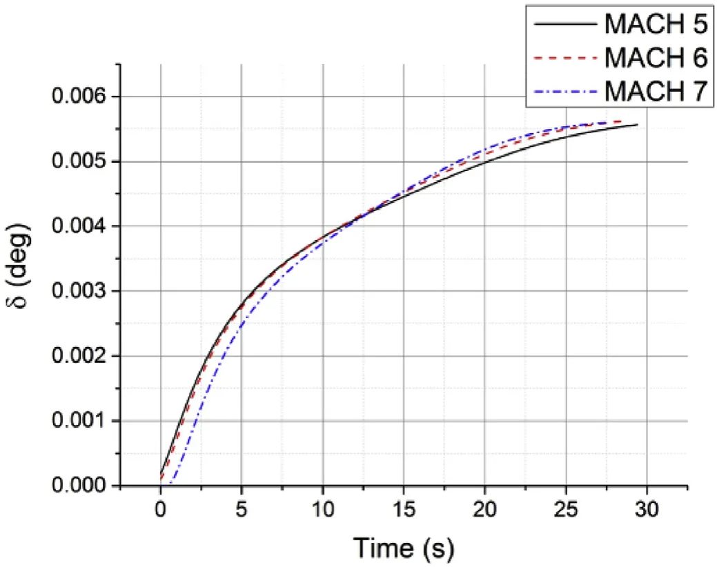
Fig.15. Pendulum angle vs. time (with ˙δ0 = 0.0573°/s).
In order to determine the initial angular velocity limits for different Mach number conditions, a series of computations were completed,and the results are shown in Table 2.This represents the relationships between maximum pendulum angle δmaxand initial angular velocity ˙δ0at each Mach number. In this table, results highlighted in bold meet the pendulum angle limits (0.04°, 0.16°and 0.53°for Mach numbers 5.0, 6.0 and 7.0). In the following analysis of EM gun-projectile launching dynamics, the initial pendulum angular velocity will be an important index which will significantly affect flight stability.It should be below a certain limit in the engineering design process.
With particle ballistic simulation,the pendulum wavelength can be calculated as shown in Fig.16. As the trajectory time accumulates, pendulum wavelength curves change smoothly. And the ranges are from 490 to 530 m, 420-460 m and 340-370 m for different Mach numbers. These are all convergent which proves there is better stability for EM gun projectile configuration in contrast to regular ones.

Fig.14. Static margin vs. angle of attack.
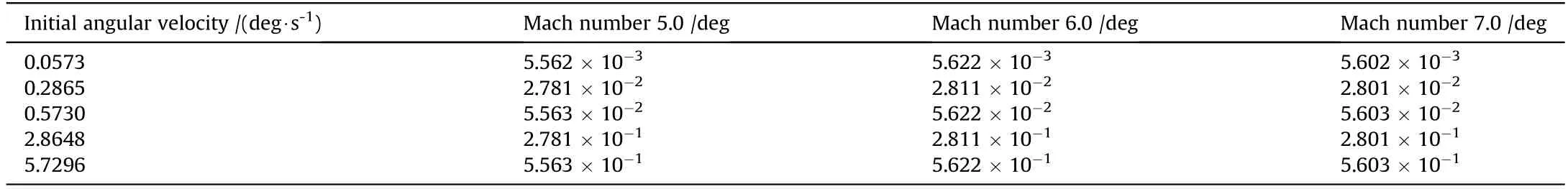
Table 2 Maximum pendulum angle δmax vs.initial angular velocity.˙δ0
Fig.16. Pendulum wavelength vs. time.
5. Conclusions
In this study, we aimed to develop a stable predictive model of EM gun launched projectiles in order to better understand the aerodynamic performance which was then compared with regular projectile layout. Based on the theory of projectile aerodynamics,the static margin and pendulum motion analysis framework were set up in order to assess the flight stability of the new airframe configuration. Using CFD analysis, it was proven that the optimization structure of EM gun projectiles performed much steadier during flight.
According to the simulation results, the static coefficients and pendulum characteristics were shown to clearly reflect the basic aerodynamics of EM gun projectiles. For static margin, regular projectile structure could barely meet the 10% requirement for stable-flight judgement. From Mach number 5.0 to 7.0, they were all greater than 10% for EM gun projectiles. With aerodynamic layout majorization, there were increments from 8.47% to 22.93%for static margin at different Mach numbers. Furthermore, drag coefficient, lift coefficient and pitch moment coefficient changed reasonably according to variations of Mach numbers and angles of attack.This illustrated that the new designed airframe acted ideally during steady state simulation. For pendulum analysis, the pendulum angle limits were set up to advise the EM gun launching system dynamics analysis and engineering design. Pendulum wavelengths of the projectile launched at different initial velocities were calculated. The convergent curves illustrated the favourable stability for configuration optimized projectiles.
Declaration of conflicting interests
The author(s) declared no potential conflicts of interest with respect to the research, authorship, and/or publication of this article.
Funding statement
This work was supported by Youth Science and Technology Research Fund, Shanxi Province Applied Basic Research Project[grant number 201801D221039], Science Foundation of North University of China [grant number XJJ201813] and Scientific and Technologial Innovation Programs of Higher Education Institutions in Shanxi [grant number 2019L0570] and Aeronautical Science Foundation of China [grant number 2019020U0002].
Nomenclature
B static margin
b a parameter which is associated with the projectile aerodynamics
Cddrag coefficient
Cllift coefficient
Cxaxial force coefficient
g acceleration of gravity, m/s2
h distance from CG to CP, m
Jyequatorial rotary inertia, kg·m2
l reference length of the airframe, m
Mzstabilizing moment,N/m
mzpitch moment coefficient
s ballistic arc length, m
S maximum cross section of projectile, m2
t flight time, s
V0projectile initial velocity, m/s2
V projectile flight velocity, m/s2
xCGaxial position of CG, m
xCPaxial position of CP,m(the positive direction of x is from the projectile nose to base)
φ included angle between the ballistic tangent and horizontal line, rad
δ pendulum angle, rad
δm0pendulum angle greatest amplitude, radprojectile initial pendulum angular velocity out of the muzzle, rad/s
λ pendulum wavelength, m
ρ air density,1.2063 kg/m3

- Defence Technology的其它文章
- Analysis of sliding electric contact characteristics in augmented railgun based on the combination of contact resistance and sliding friction coefficient
- Synergistic effect of hybrid Himalayan Nettle/Bauhinia-vahlii fibers on physico-mechanical and sliding wear properties of epoxy composites
- Study on dynamic response of multi-degree-of-freedom explosion vessel system under impact load
- An investigation on anti-impact and penetration performance of basalt fiber composites with different weave and lay-up modes
- Modeling and simulation of muzzle flow field of railgun with metal vapor and arc
- Path planning for moving target tracking by fixed-wing UAV