
Oscillation quenching and physical explanation on freeplay-based aeroelastic airfoil in transonic viscous flow
2023-11-10 02:15YyunSHIShunHEGoweiCUIGngCHENYnLIU
CHINESE JOURNAL OF AERONAUTICS 2023年10期
Yyun SHI, Shun HE, Gowei CUI, Gng CHEN, Yn LIU
a State Key Laboratory for Strength and Vibration of Mechanical Structures, School of Aerospace Engineering, Xi’an Jiaotong University, Xi’an 710049, China
b School of Aeronautics, Northwestern Polytechnical University, Xi’an 710072, China
c Beijing Institute of Structure and Environment Engineering, Beijing 100076, China
d Shenyang Aircraft Design Institute, Shenyang 110036, China
KeywordsFreeplay;
Abstract Limit Cycle Oscillation(LCO)quenching of a supercritical airfoil(NLR 7301)considering freeplay is investigated in transonic viscous flow.Computational Fluid Dynamics(CFD)based on Navier-Stokes equations is implemented to calculate transonic aerodynamic forces.A loosely coupled scheme with steady CFD and an efficient graphic method are developed to obtain the aerodynamic preload.LCO quenching phenomenon is observed from the nonlinear dynamic aeroelastic response obtained by using time marching approach.As the airspeed increases, LCO appears then quenches, forming the first LCO branch.Following the quenching region, LCO occurs again and sustains until the divergence of the response, forming the second LCO branch.The quenching of LCOs was addressed physically based on the aerodynamic preload and the linear flutter characteristic.An‘‘island”of stable region is observed in the flutter boundary,i.e.the flutter speed versus the mean Angle of Attack(AoA).The LCO quenches when the aerodynamic preload crosses this stable region with the increasing of airspeed.The LCO quenching of this model in transonic flow is essentially induced by destabilizing effect from aerodynamic preload,since the flutter speed is sensitive to AoA due to aerodynamic nonlinearity.
1.Introduction
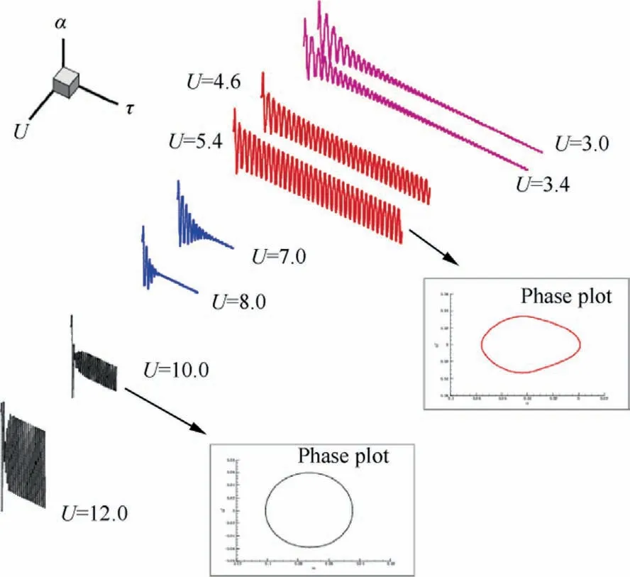
The Limit Cycle Oscillation(LCO)behavior of freeplay-based aeroelastic airfoil has been intensively studied for years in subsonic,1,2transonic3–5and supersonic6,7air flow.Based on the subsequent aeroelastic wind tunnel experiment at Duke University and continuous efforts on numerical stimulation from world-wise researchers, the nature or physical explanation of the subsonic LCO behavior induced by freeplay is becoming clear.8,9It is found that the aerodynamic preload can quench the LCO of the freeplay-based aeroelastic system below the linear flutter speed in subsonic flow, as shown in Fig.1.An obvious feature of these cases is that structural nonlinearity, i.e.freeplay, dominates the aeroelastic system,but aerodynamic nonlinearity is weak.Therefore, an interesting idea may arise as to how the freeplay-based aeroelastic system will behave if it is subjected to strong aerodynamic nonlinearity.
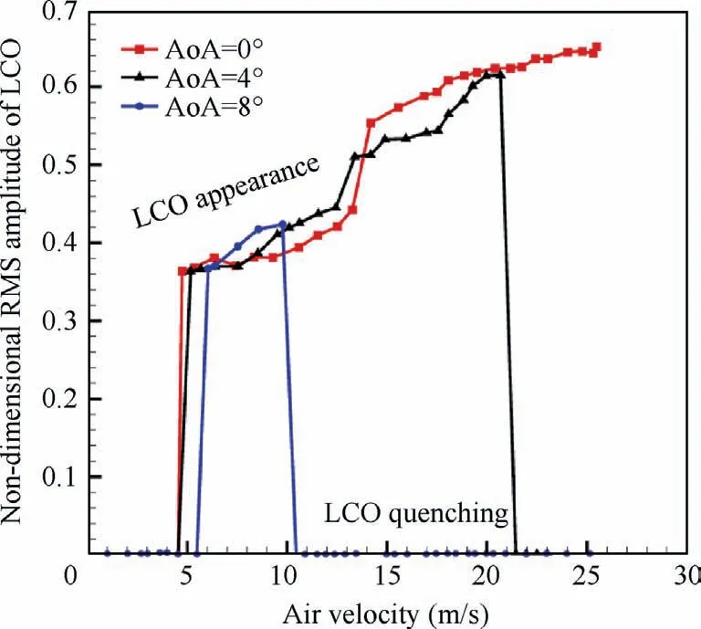
Fig.1 Illustration of LCO quenching caused by aerodynamic preload (data extracted from Ref.8).
It is well known that transonic aeroelastic system has a distinguishing feature of strong aerodynamic nonlinearity especially for supercritical airfoil in viscous flow,7,10,11due to the fact that the boundary layer of a cambered airfoil including supercritical airfoil is prone to separation with the interaction with shock in transonic flow.Supercritical airfoil NLR 7301,for example, was investigated in wind tunnel experiments12,13and numerical simulations,10,14,15displaying Hopf bifurcation even under small Angles of Attack (AoAs).Apart from these early investigations,aeroelastic behavior of supercritical airfoil draws attentions again in recent years.Hebler and Braune16–18conducted systematic experiments on the transonic flutter and LCO characteristics of supercritical laminar airfoil,denoted as CAST 10-2.Free transition flutter, heave-pitch coupled LCO and Single Degree of Freedom (SDOF) LCO were observed,16,17and subcritical bifurcations and hysteretic response with the control parameter of Mach number occurred on this aeroelastic system.18These results obtained from this supercritical airfoil reveal that the AoA normally omitted in conventional analysis plays significant effect on the nonlinear response when flow separation happens.An improved harmonic-balance-based one-shot method is developed by Li and Ekici19for LCO analysis in transonic viscous flow.‘‘Hysteresis” solution, stable and unstable branches of LCO were presented for NLR 7301 aeroelastic system in their work.Recurrent neural networks are used by Wang et al.20to build aerodynamic reduced order model for a pitching and plunging NLR 7301 airfoil in transonic flow, and generalization ability of this model was tested in predicting scalar and distributed flow variables.An improved nonlinear state-space modeling approach is proposed by Liu and Gao21to predict the transonic behavior of aircraft structure, and LCOs of NLR 7301 airfoil were used to validate their method due to the strong nonlinearity.
On the other hand, the aeroelastic airfoil considering both aerodynamic and structural nonlinearities has attracted researchers for decades,3,4,22–24but symmetrical airfoils are normally assumed and employed, which are inherited from subsonic aeroelasticity.Based on Euler equations,Yang et al.5investigated the LCO behaviors of an aeroelastic airfoil of NACA 64A010 with freeplay at different Mach numbers.An interesting chimney region was displayed in the flutter boundary.Considering a typical section of NACA 0012 profile, a three-degree-of-freedom aeroelastic airfoil with freeplay in the control surface was investigated by Candon et al.22,23using Euler-based CFD method in transonic regime.In their work,higher-order spectra techniques23and Hilbert-Huang transform techniques22were applied to understand the features and physical reasons of observed transition between different types of nonlinear aeroelastic responses.The nonlinear dynamic behavior of a NACA 64A010 aeroelastic system with freeplay in pitching Degree of Freedom (DOF) was investigated by He et al.25,26using time-marching approach based on CFD.Their results showed the type of nonlinearity dominating the nonlinear response depends on the amplitude of motion,25and roles of aerodynamic viscosity were identified in different Mach number ranges with the help of various aeroelastic analysis techniques.26
From aforementioned studies, it is easy to find that symmetrical airfoils are normally employed in considering both aerodynamic and structural nonlinearities.Nevertheless, this conventional simplification may miss aerodynamic preload effects9and the corresponding LCO quenching phenomenon in transonic flow.In addition, the transonic aeroelastic analysis on a cambered airfoil such as NLR 7301 was always limited to the linear structure.Few instances of supercritical airfoil with nonlinear structural stiffness have been reported in the existing literature.Therefore, the aim of present paper is to give an insight of the freeplay-induced LCO behavior of a supercritical airfoil subject to strong aerodynamic nonlinearity in transonic viscous flow, mainly focusing on the appearance and quenching of LCOs caused by aerodynamic preload.
The remainder of this paper is organized as follows.In Section 2, a brief introduction of the governing equations of motion and technical methods are reviewed.Section 3 presents aeroelastic behavior of an aeroelastic system with NLR 7301 supercritical airfoil and the effort to explain the observation as well.Finally, conclusions are drawn in Section 4.
2.Brief introduction of formulas and numerical method
2.1.Aeroelastic model
A classical aeroelastic airfoil with plunging(h)and pitching(α)DOFs is used in the present study as shown in Fig.2.The equation of motion of this model has already well built in existing literatures, written as
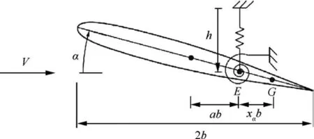
Fig.2 An aeroelastic airfoil in transonic air flow.
and detailed definition of each parameter and following nondimensional parameter can be found in Appendix.Freeplay nonlinearity is assumed in the pitching DOF herein, and the nonlinear structural restoring moment M(α) is described as
where δ denotes the freeplay angle.Eq.(1) can be written in the non-dimensional form as
where (∙)′=d(∙)/dτ,(∙)′′=d2(∙)/dτ2.Subsequently, the governing equation can be written in matrix form:
2.2.CFD-based time marching simulation
The time marching approach based on CFD technique is a high-fidelity method to calculate the aeroelastic response in transonic air flow.In our previous study,26a tool based on Ansys Fluent and its User-Defined Functions(UDF)has been well developed and validated.In Fluent, a control-volumebased technique is employed to convert the general scalar transport equation to an algebraic equation, which is solved by using a point implicit (Gauss-Seidel) linear equation solver in conjunction with an Algebraic Multigrid (AMG) method.The S-A model is used to deal with viscous flow problems.For spatial discretization, the second-order upwind scheme is utilized to interpolate the convection terms.In terms of temporal discretization, bounded second order implicit time integration is employed for real-time advancement to carry out the unsteady flow field.
In this tool, the mesh deformation model using Radial Basis Function (RBF)27,28is implemented to enhance the capability of mesh deformation.Fourth-order Runge-Kutta(RK4) and aerodynamic interpolation technique is programmed, which is helpful in reducing the sensitivity of time step on time marching simulations.26Since freeplay nonlinearity is analyzed in the current paper, Henon method is used to accurately detect the crossover and switch the integration in different linear sub-domains precisely.26,29
To show the capability of present tool in simulating aeroelastic response in transonic viscous flow, LCOs of NLR 7301 airfoil caused by nonlinear aerodynamics are obtained in this section.The structural parameters are taken from Refs.10,30based on the original experimental model.0°freestream AoA was assumed when performing time marching simulations.After repeating the simulation at individual airspeeds, the amplitude and frequency of the aeroelastic response were extracted and plotted against the airspeed, also known as the LCO behavior.
Fig.3 shows the computed LCO behaviors (nondimensional speed is used in the current paper).It can be seen that the linear flutter speed is around U=5.0,and simple LCO occurs when the airspeed is slightly increased.Comparisons in Fig.3 show that of LCO solutions obtained by the present method agree well with our previous aerodynamic describing function method,30the harmonic balance method10and its recent improved approaches,19,31revealing the high accuracy of the present time marching method based on CFD.
2.3.Static aeroelastic solution
2.3.1.Coupled scheme with steady CFD
Since an unsymmetrical airfoil is adopted in the current paper,the static aeroelastic position would be non-zero due to aerodynamic moment.As demonstrated in our previous study,25the static aeroelastic position, also called as aerodynamic preload,8,9can alter the type of the structural nonlinearity to a freeplay with preload.Thus, it is important to find the solution for the static aeroelastic position.
Neglecting the time-dependent terms in Eq.(4),the governing equation for static aeroelasticity can be expressed as
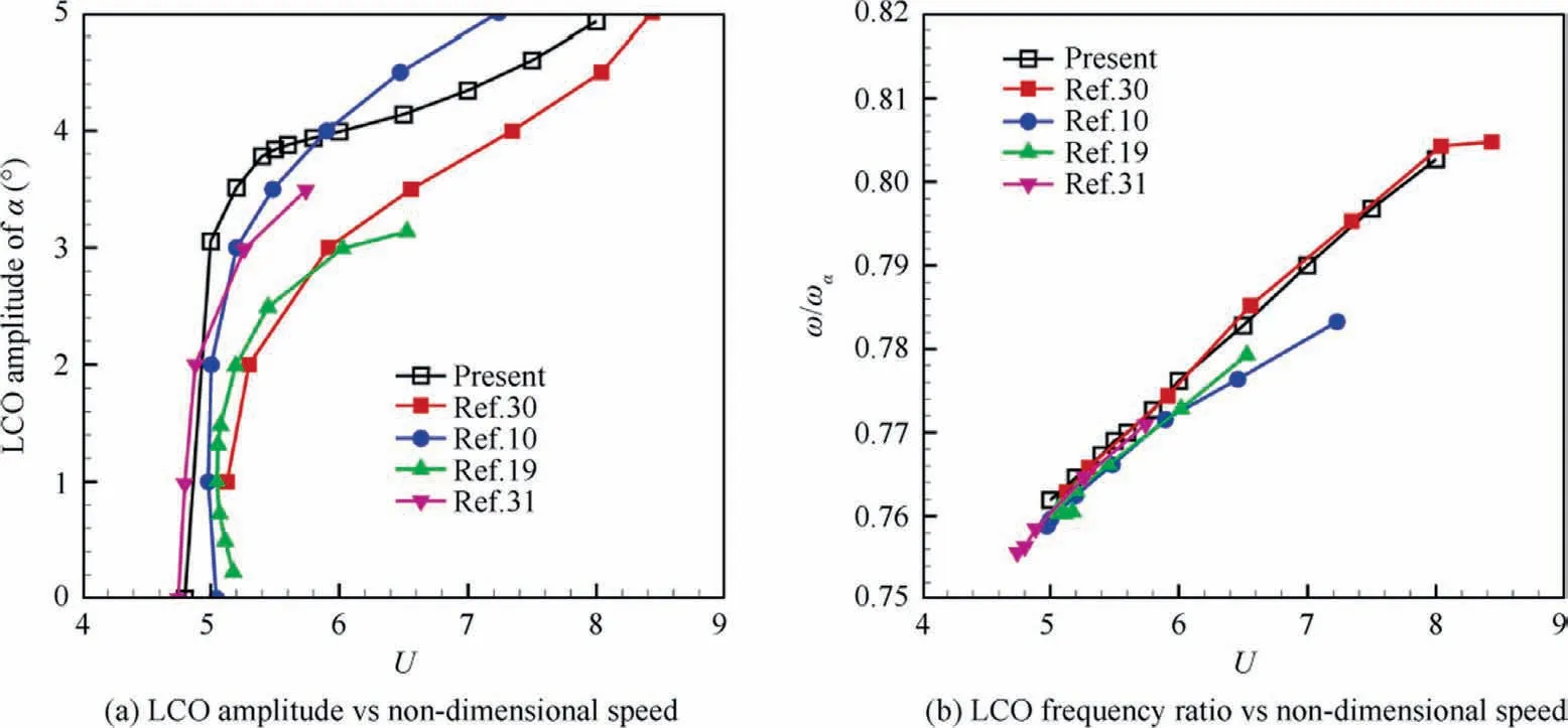
Fig.3 Comparison of LCO behaviors for NLR7301 configuration with linear structural model.
Obviously,it is a nonlinear equation due to nonlinear term Fnoncaused by the freeplay.Once the aerodynamic forces faare carried out from steady CFD calculation, the displacement vector ξ will be obtained by using the fixed-point iteration to solve the above structural equation.
Thus, a loosely-coupled method between steady CFD solver and nonlinear structural equation is developed to achieve the static equilibrium aeroelastic position.The process can be described as:
(1) Run steady CFD simulation to obtain aerodynamic force coefficients fa.
(2) Solve nonlinear equation,Eq.(5),to obtain the displacement in plunging and pitching DOFs.
(3) Update mesh according to the calculated displacement,and repeat (1)-(3) until the displacement of the governing equation converges,i.e.the static aeroelastic equilibrium position.
2.3.2.Graphical method
An efficient method to obtain the static aeroelastic equilibrium is developed via the graphic method in this section.Since plunging motion plays little role on steady aerodynamic forces,the plunging DOF of Eq.(5) can be neglected, yielding
or
The graphic method is adopted to solve the above nonlinear equation, and the procedure is as follows.The aerodynamic moment coefficient at different freestream AoA is obtained by repeating the steady CFD simulations individually.The Cmcurve representing the right hand of Eq.(7) can be drawn by depicting the aerodynamic moment coefficient over α.The left hand of Eq.(7), i.e., can be determined by specify airspeed U and freeplay angle δ, and then becomes a univariate function of α.Drawing these two curves F(α) and Cmtogether, the point of intersection turns out to be the static aeroelastic solution.
2.4.Linear flutter characteristic at predefined mean AoA
2.4.1.Time marching approach
It is important to work out the flutter speed at a predefined AoA αmin the present study.The CFD-based time marching simulation technique is developed to force the aeroelastic response vibrating around the fixed AoA.
As the mean AoA is specified, the pitching motion can be described as
where Δα is perturbation of pitching motion around αm.Removing the nonlinear term fnonin Eq.(3) for the linear structure and substituting Eq.(8) into it, the governing equation of this case is built as
From Eq.(6),the static aeroelastic equation of linear structure at αmcan be expressed as,
where Cm0is the aerodynamic moment coefficient at AoA of αm.To cancel term of αm, Eq.(10) is substituted into Eq.(9)leading to the governing equation of motion at the fixed AoA,
Same to the conventional time marching approach,the flutter solution can be found by observing the time history of Δα at a series of airspeeds.
2.4.2.Frequency domain method
As an alternative to obtain the linear flutter characteristic of the aeroelastic model at specific AoA, the Aerodynamic Influence Coefficient (AIC) and frequency domain flutter solution are employed in the present study.
Based on the authors’ previous work,5,30CFD can be regarded as an implicit system with the generalized displacements as inputs and the generalized aerodynamic forces as output.The aerodynamic influence coefficient is the ratio of the first order harmonic component of the complex output and the harmonic input.Thus, the generalized aerodynamic forces associated with the airfoil motion can be written as
where Q is the AIC matrix,which is related to mean AoA(αm),Mach number (Ma) and reduced frequency.The detailed process to build the aerodynamic influence coefficient can be found in Ref.30
Applying linear structural model and with the flutter condition of harmonic motion ξ= ξ0eiωt, the combination of Eq.(4) and Eq.(12) yields the transonic linear flutter equation in frequency domain
For a prescribed Mach number or AoA, several transonic AIC matrices can be carried out for different reduced frequencies.Then the transonic linear flutter equation,Eq.(13),can be solved using the conventional frequency domain flutter analysis method such as p-k method.Linear flutter speed and linear flutter frequency at this Mach number or AoA are obtained subsequently.
The widely used benchmark, Isogai wing,32is employed in the section to show the fidelity of the present transonic AIC method and time marching approach with CFD.The flutter boundary is obtained and illustrated in Fig.4 by depicting the flutter speed and frequency versus Mach number.The results obtained by both the time marching approach based on CFD33–35and the present transonic AIC method are in good agreement.From Fig.4(a), it can be seen that flutter speed in the transonic regime is obviously lower than those in the subsonic regime, which is usually termed as ‘‘transonic dip”.Moreover, there are multiple values of flutter speed between Mach 0.85 and 0.9, which form the so-called S shape flutter boundary.36Note that the same technique was used in our previous investigation37for the feasibility of this method.
3.Numerical results and discussion
The aeroelastic system with NLR 7301 supercritical airfoil is studied, where the freeplay nonlinearity is assumed in the pitching DOF.The relevant parameters used are xα=0.555,r2α=0.822, μ=172, ωh/ωα=1.83, a=-0.5, ζh=0.0175,ζα=0.00411.The computed Mach number is 0.75, and the sea level air condition is adopted, so the resulting chord Reynolds number is 1.75×10⁷.
The grid independence study and time step convergence study were carried out as the same manner as our previous study.26A C-type grid is adopted as shown in Fig.5.The outer boundary of the computational domain extends to a distance of 50c from the airfoil surface, and the first layer thickness of all these grids is set to 3×10⁻⁶c, with y+<1 on the airfoil surface.Basically, three different mesh resolutions were used to run unsteady CFD simulation at Mach 0.75 excited by a sinusoidal pitching oscillating motion.Discrepancy of the time history of the unsteady aerodynamic coefficient for different meshes were compared and used to select the proper mesh.Finally, a medium size of mesh with 60800 elements (468 points on the airfoil, 71 points in flow wake, 101 points in radial direction) was applied in the following sections.
Since the aerodynamic interpolation technique is used in our CFD simulation tool, the sensitivity of time step in time marching simulations reduces.26A series of time-step sizes were used, and the calculated responses from different time steps converge as the time step decreases.The good agreements of pitching response from Δτ=0.04 to Δτ=0.01 are observed.To balance the computational cost and accuracy,Δτ=0.04 was adopted in our following simulations.
3.1.Nonlinear dynamic responses
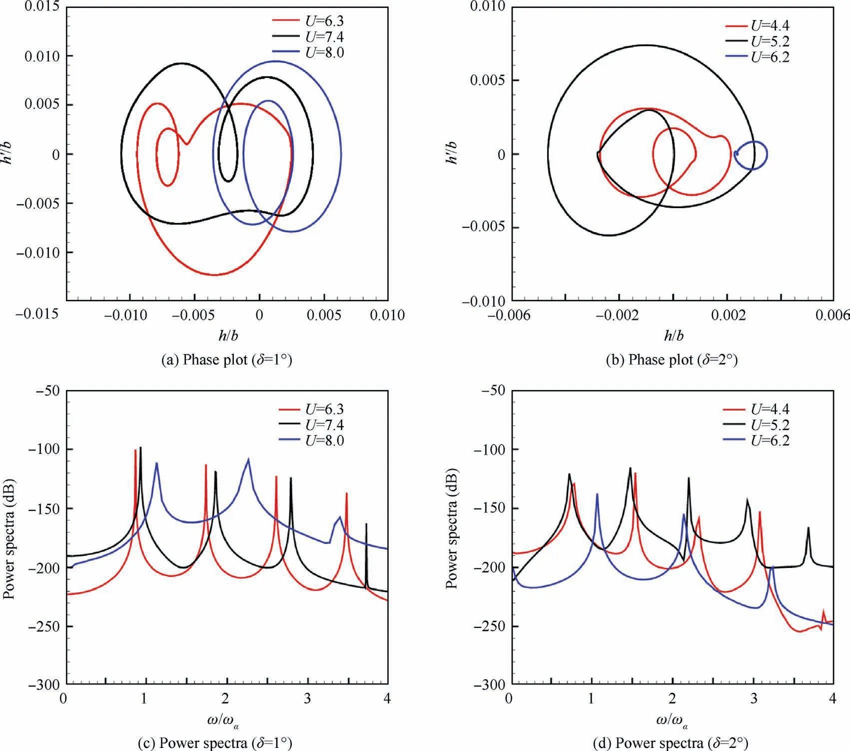
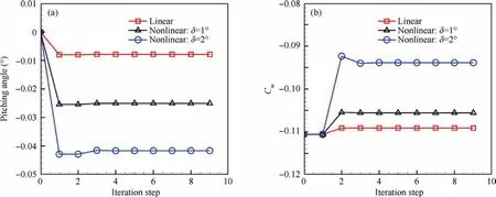
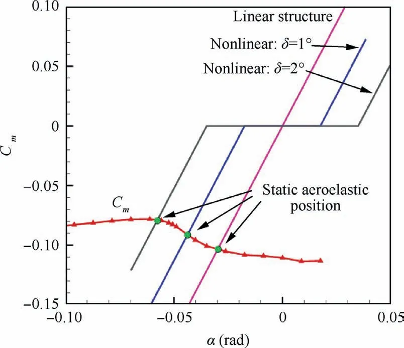
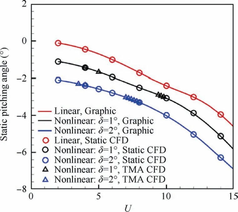
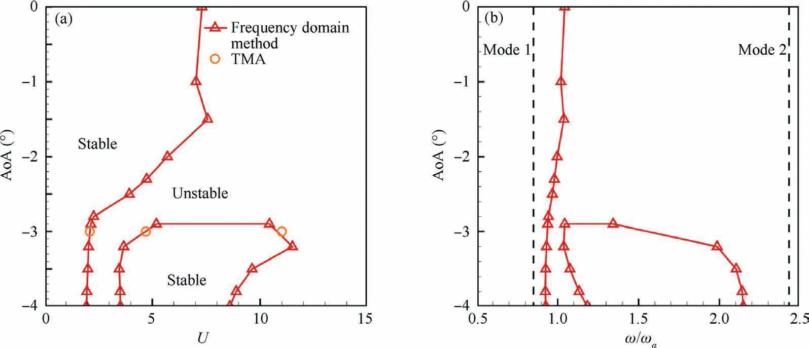
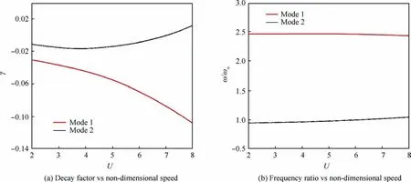
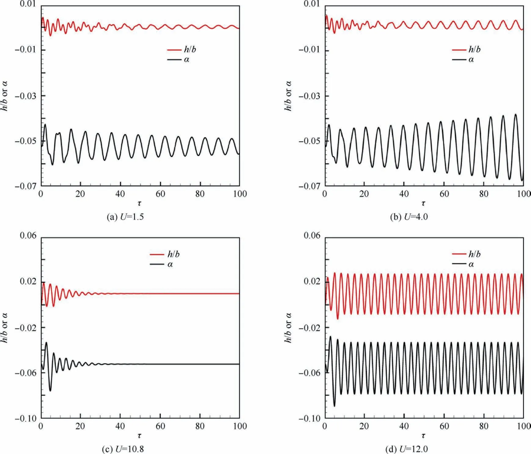
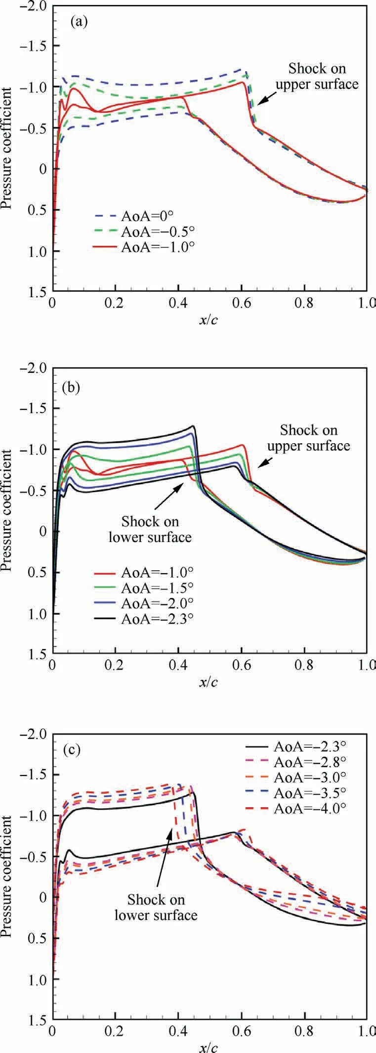
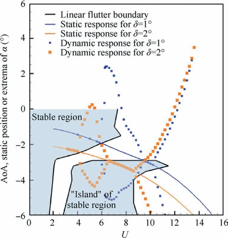
Fig.6 shows the bifurcation diagrams for NLR 7301 with freeplay(δ=1°and δ=2°).For both cases,it is observed that as the non-dimensional speed U increases, the LCO appears firstly and then quenches.When the speed is increased further,LCO motion occurs again and sustains until the divergence of the response.The speed range for LCO quenching is 9.4 Several typical time histories of pitching are plotted in Fig.7 to illustrate this interesting phenomenon.Only simple harmonic motions,i.e.simple LCOs,were observed in pitching motion on both LCO branches from phase plots in Fig.7.Unlike pitching motion,the plunging responses are more complicated in the first LCO branch in 6.0 Fig.6 Bifurcation diagrams for NLR 7301 airfoil with freeplay of (a)(b) δ=1° and (c)(d)δ=2°. Fig.7 Aeroelastic responses of pitching at typical non-dimensional speeds for δ=2°. It has been noticed that amplitudes of plunging DOF are obviously different on the first/second LCO branch from the bifurcation diagram in Figs.6(b) and (d).To show the contribution of plunging motion more clearly,the amplitude ratio of plunging and pitching motion (h0/(α0b )), which can be regarded as an equivalent of flutter mode shape,30are used and compared in Fig.9.It is found that h0/(α0b ) is less than 0.22 on the first LCO branch, while it is larger than 0.83 on the second branch.It can be inferred that pitching motion dominates the aeroelastic system in the first LCO branch,while LCOs on the second branch are results of coupling between pitching and plunging motion. Referring to Refs.8,9,25, preload angles (static aeroelastic position) and linear flutter speeds play significant roles in the freeplay-induced aeroelastic responses.In the following sections, the quenching of LCOs will be addressed based on the static aeroelastic analysis and linear flutter speed for different AoAs. As mentioned in Section 2.3.1, the loosely-couple method based on steady CFD solver and static structural equation can be used to obtain the static aeroelastic position.Fig.10 shows iteration process of the pitching angle and aerodynamic moment coefficient at U=4.It is observed that the coupled system reaches its static equilibrium position after around 3 iteration steps.In addition, it is also found the static pitching angle depends on the structure properties, such as the linear structure or nonlinear ones with different freeplay angles (δ).But in general, the magnitude of aeroelastic equilibrium increases when the freeplay angle increases. Fig.8 Typical aeroelastic responses of plunging motion in first LCO branch. Fig.9 Contribution of pitching and plunging on LCOs. Graphic method was also used to obtain nonlinear static position, the process of which is illustrated in Fig.11.From this figure,the reason why the larger freeplay angle δ leads to a large magnitude of static aeroelastic pitching angle can be easy understood.Furthermore,it can also be inferred that the static aeroelastic equilibrium would be always negative for a cambered airfoil because of the nose-down pitching moment.In addition, the static aeroelastic positions obtained from the above two approaches are compared with time marching approach in Fig.12.Good agreement is observed, indicating the accuracy of these methods used in the present study. To sum up,as the airspeed increases,the magnitude of static aeroelastic pitching angle increases quadratically.For the case of δ=2°, the maximum magnitude of static aeroelastic angle can be as large as 7°.Theoretically speaking, such large mean AoA would significantly affect the flutter characteristic of the aeroelastic system in transonic flow, which will be addressed in the next section. The influence of aeroelastic equilibrium on the wing transonic flutter characteristic was evaluated by using transonic AIC method as follows.The freestream AoA of the NLR 7301 model was set to a specific value in CFD solver when calculating aerodynamic influence coefficients.Then the wing transonic flutter characteristics at this AoA can be obtained by frequency domain flutter analysis method. Fig.10 Evolution of (a) pitching angle and (b) aerodynamic moment coefficient for linear/nonlinear structural model at U=4. Fig.11 Graphic method to solve static aeroelastic equation at U=8. Fig.12 Static aeroelastic position for different airspeed U for linear and nonlinear structures (TMA is short for time marching approach based on CFD). As shown in Fig.13(a), the flutter speed is plotted against AoA in the range of 0°--4°.An interesting S shape flutter boundary with varying AoA is observed.The S shape flutter boundary was once used to show the special shape of Isogai wing model’s flutter boundary,but the flutter speeding is plotted against Mach number as shown in Fig.4.It is also found that the flutter frequencies for the lower flutter speed, as marked in Fig.13(b), are close to the first natural frequency,implying the single degree of freedom flutter.38 The S shape flutter boundary can be explained by observing the system stability in different airspeed ranges.In the present NLR 7301 model, within the AoA range of 0°--2.8°, a single flutter speed is detected.For the case of AoA=-1°as shown in Fig.14, a conventional bending-torsion coupling flutter is observed, and the flutter speed is 7.0.When the magnitude of AoA increases above 2.9°,multiple flutter speeds take place at each AoA.At AoA = -3.2° as shown in Fig.15, a hump mode from the first aeroelastic mode occurs.In this case, the aeroelastic system is stable at U<2.01.As the airspeed increases, the system becomes unstable at 2.01 To further verify the existence of multiple flutter speeds in this model,time marching method based on CFD for aeroelastic response simulation at a fixed AoA, as mentioned in Section 2.4.1, is performed.Taking AoA = -3°as an example,several typical aeroelastic responses are selected to show the aeroelastic stability in different speed regions at this AoA.In the speed range U<2.1, a damped motion is observed as shown in Fig.16(a).In 2.1 Finally, flutter speeds at predefined AoAs obtained by observing aeroelastic response are compared with the above frequency domain method based on transonic AIC method in Fig.13.Good agreement from both methods is observed,revealing the occurrence of multiple flutter speeds in this nonlinear aeroelastic model. Fig.13 (a) Flutter speed and (b) flutter frequency at different AoA. Fig.14 Decay and frequency characteristics of aeroelastic system at AoA = -1°. Fig.15 Decay and frequency characteristics of aeroelastic system at AoA = -3.2°. As we know, the transonic flutter characteristic is closely related to the shock location.Steady flow fields at different AoA of 0°--4°are examined in this section.The pressure coefficient was obtained by steady CFD simulation and plotted in Fig.17 From Fig.17(a),it is found when magnitude of AoA is less than 1°, the shock locates on the upper surface of the airfoil.As the magnitude of AoA increases from 1° to 2.3°, the shock on the upper surface weakens and the one on the lower surface emerges.Thus, shocks locate on both sides of the airfoil as shown in Fig.17(b).When increasing further to 4°, the shock on upper surface disappears,while the one on the lower side dominates the flow field and moves towards the leading edge of the airfoil.The correlation between the shock location and the flutter speed in this case with a supercritical airfoil is much more complicated than that of a symmetric airfoil.37This might be caused by the SDOF flutter as we mentioned above. Fig.16 Aeroelastic response at mean AoA = -3°of linear structure. Fig.18 depicts the flutter boundary, nonlinear static aeroelastic position (aerodynamic preload angle) and nonlinear dynamic response together.Thus, the quenching of LCOs can be easily explained as the following manner.The stability of aeroelastic system alters as the airspeed goes up.The aeroelastic system normally becomes unstable when the airspeed increases.Particularly, an ‘‘island” of stable region happens for the present model.It is clear that as the airspeed increases,the magnitude of static aeroelastic angle increases.When the magnitude of mean AoA is large enough, the aeroelastic system leaves the stable region and enters the unstable region,so the first LCO branch appears.With further increasing of airspeed, the aeroelastic system departs from the unstable region and goes into another stable region.Therefore, the quenching of LCO takes place when the system crosses the stable region.As the airspeed increases further, the aeroelastic system becomes unstable again and the second branch of LCO emerges. From the static aeroelastic and linear flutter analysis, the airspeed region for LCO quenching can be predicted as 9.44 As reported by Kholodar8and Padmanabhan9et al., the LCO quenching is essentially induced by destabilizing effect of aerodynamic preload on aeroelastic system.From this perspective, the present transonic scenario is identical with their conclusion.It should be pointed out that such destabilizing effect in transonic flow is actually induced by the mean AoA effect on the flutter speed due to the aerodynamic nonlinearity,while freeplay nonlinearity mainly acts on the static aeroelastic position.Nevertheless, in subsonic cases it is the nonlinear stiffness from structural nonlinearity, namely freeplay, that leads to the instability of the aeroelastic system. Fig.17 Pressure distribution at different AoA of NLR 7301 at Ma = 0.75. Fig.18 Explanation of LCO quenching in freeplay-based aeroelastic system in transonic flow. Based on the Navier-Stoke equations, the nonlinear behavior of an aeroelastic system with NLR 7301 supercritical airfoil assuming freeplay in pitching DOF is studied in transonic air flow.Time marching approach is used to obtain the nonlinear aeroelastic response.A loosely-coupled steady CFD /structural equation method and a graphic method are developed to obtain the static aeroelastic position (or aerodynamic preload) caused by the non-zero aerodynamic moment due to unsymmetrical airfoil.The transonic AIC method and the time marching approach are used to obtain the linear flutter characteristic at specific mean AoA. An interesting LCO quenching phenomenon is observed in the bifurcation diagram.Nonlinear aeroelastic behavior can be described as:with the increasing of airspeed,the LCO appears firstly and then quenches; when the airspeed is increased further, the second LCO branch occurs until the divergence of the response.To explain this observation, following investigation is carried out: the static aeroelastic position is obtained,and the magnitude of static aeroelastic pitching angle increases quadratically with the increasing of the airspeed; the flutter speed at different AoA is examined, and an S shape flutter boundary with varying AoA is observed. The appearance and quenching of LCOs are the result of combined action of the static aeroelastic position caused by cambered airfoil and the S shape flutter boundary with respect to AoA.As the airspeed increases, the static aeroelastic position changes, hence the stability of aeroelastic system alters.When the aeroelastic system leaves the first stable region and crosses the unstable region, the first LCO branch appears.With further increasing of airspeed, the aeroelastic system departs from the unstable region and enters the ‘‘island” of stable region, leading to the LCO quenching.When the airspeed is increased large enough, the aeroelastic system becomes unstable again and the second branch of LCO takes forth.This study provides a useful approach to evaluate the effects of the control surface freeplay on aeroelastic characteristics of an aircraft due to aerodynamic preload especially in transonic flow. The LCO quenching is essentially induced by destabilizing effect of aerodynamic preload on aeroelastic system.Such effect in transonic flow is mainly caused by the sensitivity of flutter speed on AoA due to the aerodynamic nonlinearity,while freeplay have an impact on the static aeroelastic position. Declaration of Competing Interest The authors declare that they have no known competing financial interests or personal relationships that could have appeared to influence the work reported in this paper. Acknowledgement The authors acknowledge the financial support by the National Natural Science Foundation of China (No.12102317). Appendix A.As shown in Fig.2, the elastic axis of the airfoil locates at E point in at a distance of ab rear of the mid-chord point.The gravity center(G point)is located at xαb behind the elastic axis, where b is the half-chord length. m is the mass per unit span, Sα=mxαb is the first moment of inertia about the elastic axis, and Iα=mr2αb2is the moment of inertia about the elastic axis. Kh=mω2his the plunging stiffness coefficient, and Kα=Iαω2αis the torsion stiffness coefficient. L=ρV2bCLand Meα=2ρV2b2Cmare the aerodynamic lift and moment about the elastic axis.CLis the lift coefficient,Cmis the aerodynamic moment coefficient,ρ is the air density,and V is airspeed. τ=ωαt is non-dimensional time,μ=m/πρb2is mass ratio,U=V/bωαis the non-dimensional airspeed, and k=ωb/V is reduced frequency.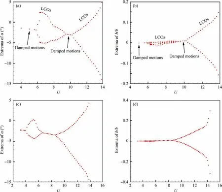
3.2.Aeroelastic static responses

3.3.Effect of mean AoA on flutter speed

3.4.Physical explanation of LCO quenching
4.Conclusions
 CHINESE JOURNAL OF AERONAUTICS2023年10期