Longitudinal mediation analysis based on Mendelian randomization*

,

School of Management, University of Science and Technology of China, Hefei 230026, China

Abstract: Instrumental variables(IVs) are widely used in mediation analysis to effectively reduce causal effect bias due to unobserved confounding factors and reverse causal direction that cannot be handled with conventional causal inference methods.Most IV methods in the literature are designed for cross-sectional studies.Longitudinal data can better reflect causal paths than cross-sectional data, which provides observations of individual patterns of changes and measurements of event duration.To our knowledge, there is no IV method specifically tailored for longitudinal mediation analysis in the literature.A new IV method is proposed to estimate longitudinal mediation effects.Large sample properties,including consistency and asymptotic normality, are established for the new IV method.Simulation studies are provided to demonstrate the desired finite sample properties of the new method.

Key words: causal inference; Mendelian randomization; mediation analysis; longitudinal data

Mediation analysis is widely used in biomedical and social sciences to investigate the mechanism underlying the effect transmission of an exposure variable on an outcome variable by an intermediate variable (i.e., a mediator) (Iacobucci,2008).Natural and controlled mediation effects have been well defined for time-independent exposures (Robins et al.,1992;Pearl,2001;Imai et al.,2010).Alternatively, lifetime mediation effects (LMEs) were defined for time-dependent exposures, which reflect mediation process by emphasizing time variations (Labrecque et al.,2019;Labrecque et al.,2020).Since cross- sectional studies cannot provide time-related information such as observations of individual change pattern and measurements of event duration, it is natural to use longitudinal data instead of cross-sectional data to estimate LMEs.

Mediation analysis suffers from unmeasured confounding factors in observational studies as either the exposure or the mediator is usually not randomly assigned, and instrumental variables (IVs) can be used to obtain a consistent estimate of the average causal effect including direct effect and mediation effect(s) in this situation(Smith et al.,2003;Hernan et al.,2006).An IV is assumed to have no any direct effect on the outcome, which means that IV should influence outcome entirely via treatment variable (Mehta,2001).In econometrics, commonly accepted IVs include aggregation data (Card et al.,1996), natural phenomena (Cipollone et al.,2007), social distance and price (Hall et al.,1999), as well as random assignment (RA) (Krause et al.,2003).These IVs suffer from some restrictions that are hard to overcome.First, RA is based on randomization experiment that could be costly or even unable to conduct, and it is hard to have two or more RAs in a single study, limiting the application of RA in mediation analysis.Second, other IVs based on observation studies could suffer from confounding factors, violating the no-direct-effect assumption.In summary, it is generally difficult to find valid IVs in practice.The method using genetic variants as IVs is referred to asMendelian randomization(MR) (Lawlor et al.,2008).According to Mendel's law of independent assortment, a polymorphism can be served as randomized proxy markers for different exposures if they are indeed associated with the exposures.MR has been widely used in causal inference studies (Grover et al.,2017) due to the popularity of genomewide association studies.MR has some extensions, such as multivariable MR (MVMR) and network MR, which have been used to estimate mediation effect in MR studies (Burgess et al.,2015;Sanderson et al.,2019).

In the literature, some MR methods have been proposed to estimate LMEs using cross-sectional data under some assumptions about time (e.g., constant genetic effect on the exposure) (Labrecque et al.,2019).However,these assumptions may be violated in practice, resulting in biased estimates of LMEs (Dumitrescu et al.,2011;Shirts et al.,2011;Neu et al.,2017).In this paper, we aim to develop a valid MR method for estimating LMEs using longitudinal data, which allows the genetic effect to be time varying.

The rest of this paper is organized as follows.Some examples are given in Section 1 to illustrate that the existing MR methods are invalid for estimating LMEs when the effects of IV on exposures are time varying while the proposed MR method provides a consistent LME estimator.The asymptotic normality of the proposed MR method is also established in this section.In Section 2, the validity and advantages of the proposed method are illustrated through extensive simulations, and the proposed MR is shown to be quite robust to the violation of required identifiability conditions through sensitivity analyses.Section 3 concludes the paper with a discussion and future research directions.

1 Methods

In this section, we first give the definition of LMEs, then show the identifiability of LMEs with MR method under some mild conditions.Next, we develop a new statistical method for inferring LMEs.Some large sample properties are established for the proposed method.

1.1 Definitions of LMEs in mediation analysis

In this subsection, we restate the definitions of lifetime average causal effects (LACEs) for simple causal inference and LMEs for mediation analysis, which were originally given in Labrecque et al.(2019) and Labrecque et al.(2020).

In the simple causal inference problem, LACEs were defined as effects of shifting the entire exposure trajectory by one unit on the outcome variable at the last observation time of the exposure.Unfortunately, LACEs cannot be consistently estimated with the traditional MR method without the assumption of constant genetic effect on the exposure.In the context of mediation analysis, LMEs can be regarded as an extension of LACEs.LMEs include lifetime total effects (LTEs), lifetime direct effects (LDEs), and lifetime indirect effects (LIEs).LTE is the effect of shifting the entire exposure trajectory by one unit on the outcome at the last observation time point; LDE is the effect of shifting the entire exposure trajectory by one unit, while holding mediator at the original state, on the outcome at the last observation time point; LIE is the effect of shifting the entire mediator trajectory by a certain amount on the outcome at the last observation time point, where the amount of mediator shifting is what the mediator would have shifted due to shifting the entire exposure trajectory by one unit.Like LACEs, LMEs cannot be consistently estimated with the existing MR method if the genetic effect on the exposure is time varying.

1.2 Traditional MR methods

Before introducing our method, we briefly review the univariable MR method and two of its extensions for mediation analysis (i.e., MVMR and 2SMR).

In univariable MR, the effect of the exposure on the outcome can be consistently estimated even when unmeasured confounders are present as long as the genetic instruments are valid (refer to Sanderson(2021) for some conditions required for the validity of univariable MR).As two extensions of the univariable MR, MVMR (Burgess et al.,2015) and two-step MR (2SMR) (Relton et al.,2012) are widely used to determine the proportion of the total effect of the exposure on the outcome that acts through particular mediators.The key idea of 2SMR is using univariable MR twice to estimate the indirect effect of the exposure on the outcome.MVMR allows for multiple exposures, and the effect of any exposure on the outcome can be consistently estimated as long as the genetic instruments are valid (refer to Sanderson(2021) for conditions required for the validity of MVMR).Generally speaking, in mediation analysis with a single time point, univariable MR estimates the total effect of the exposure on the outcome while MVMR estimates the direct effect of the exposure on the outcome.

1.3 The existing MR methods are not valid for estimating LMEs

We use a simple example to illustrate that the traditional MR method cannot consistently estimate LMEs,which is graphically depicted in Fig.1(a).This example involves two instrumental variables, one exposure and one mediator evaluated at two time points, respectively, as well as one outcome at the second time point.Specifically,GAandGBrepresent one or more genetic variants (instrumental variables),A0andA1are continuous exposures at two time points,B0andB1are continues mediators at two time points, andYis the outcome of interest.For simplicity, unmeasured confounders between the exposure and the mediator, the mediator and the outcome, as well as the exposure and the outcome, are not shown in this graph.

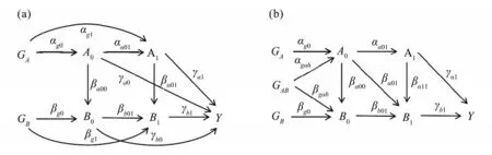
Fig.1 (a) An example of longitudinal mediation model for illustrating the definitions of LMEs;(b) The proposed longitudinal mediation effect model for estimating LMEs.

Unfortunately, the traditional MR method cannot consistently estimate LMEs if the effects of genetic instruments on the exposure or mediator are not constant (i.e.,αg0≠αg0αa01+αg1orβg0≠βg0βb01+βg1, whereαg0is the genetic effect onA0,αg1is the direct genetic effect onA1,αa01is the causal effect ofA0onA1,βg0is the genetic effect onB0,βg1is the direct genetic effect onB1, andβb01is the causal effect ofB0onB1).The traditional MR methods focus on estimating the effects of point or time-fixed exposures on the outcome using the effects of genetic instruments on the exposures and the outcome.According to the definitions, LMEs involves the entire trajectory of the exposures.Since genetic instruments affect the outcome only through the exposures as assumed in the framework of MR methods, traditional MR methods require time-independent effects of genetic instruments on the exposures to consistently estimate LMEs.In the model depicted in Fig.1(a), the effects of genetic instruments on the exposures are functions of time-varying causal effectsαt's,βt's andγt's.Consequently, the traditional MR methods specifically tailored for cross-sectional data are not valid in estimating LMEs ifαt's,βt's andγt's are time dependent.

1.4 The proposed longitudinal mediation effect model and identifiability of LMEs

We propose to use the following longitudinal mediation effect model:

whereU1,U2, andU3are unmeasured confounders between the exposure and the mediator, the exposure and the outcome, and the mediator and the outcome, respectively.GABis genetic instrument associated with both the exposure and the mediator.This model is graphically shown in Fig.1(b).In model (1), only two time points are considered for simplicity, but this model actually allows for multiple time points.

Now we consider the identifiability of LMEs in the context of model (1).In addition to the identifiability conditions required for the traditional MR method designed for cross-sectional data (Grover et al.,2017), we need some extra conditions since the genetic effects on exposures and mediators are time varying.

Assumption 1 Linearity of associations (parametric form): All the associations are linear (all the possible relationships between genetic variant, exposure, mediator, confounders, and outcome), as shown in model (1).

Assumption 2 No correlation or interaction between components of the genetic instrument: All the genetic variants are not correlated with each other and show no interaction among each other.

Assumption 3 Effect homogeneity: There is no difference in the causal effect between variables of different individuals.

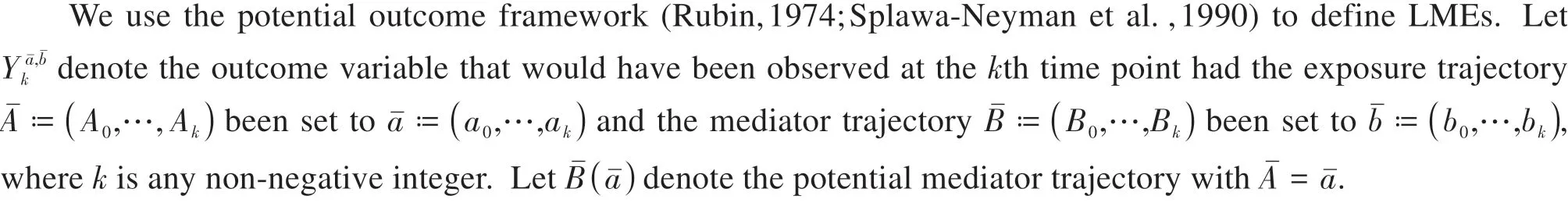
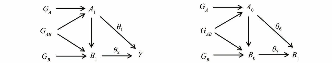
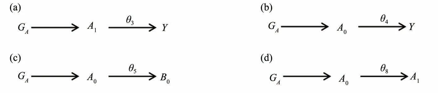
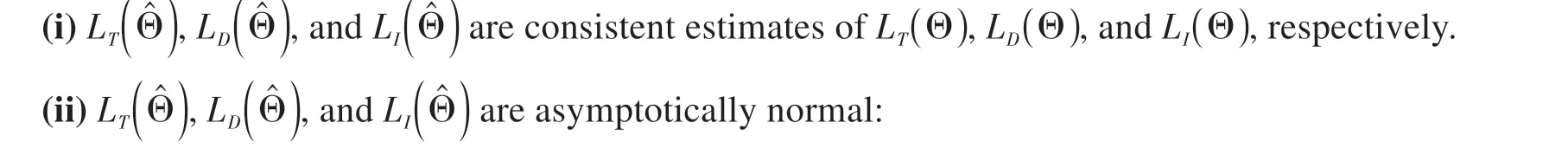
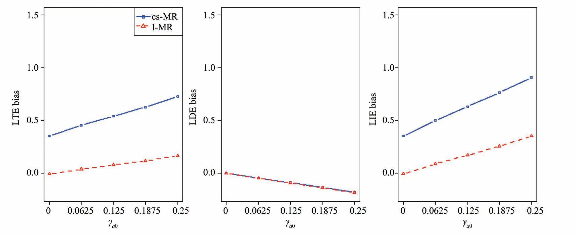
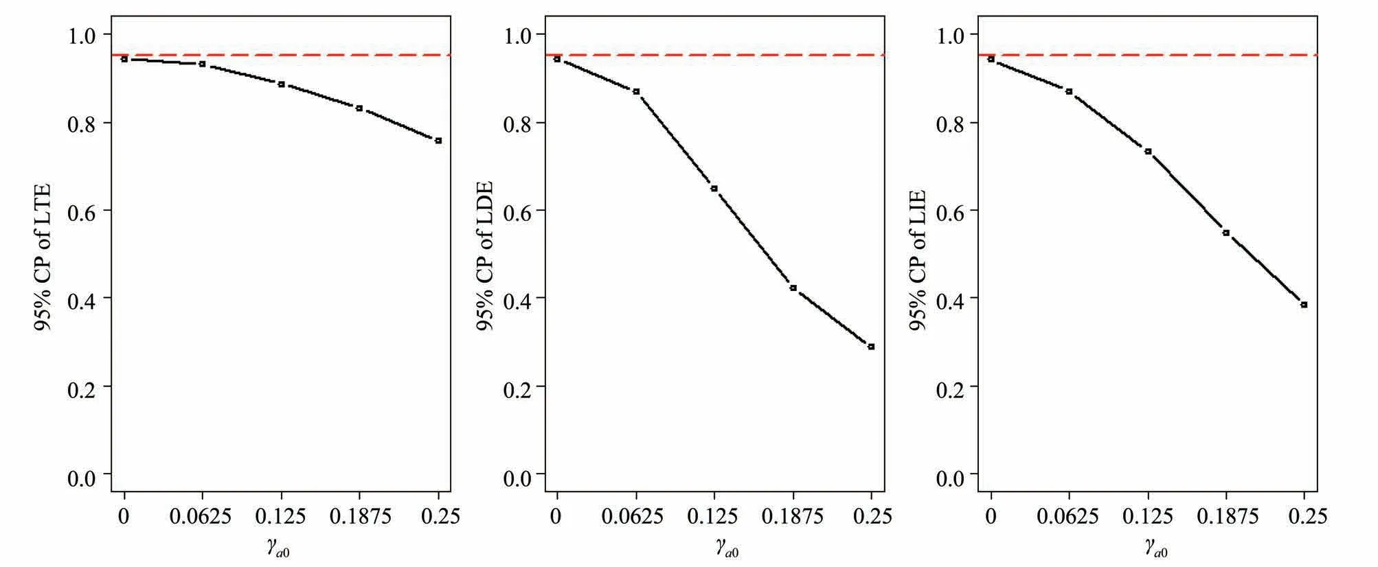
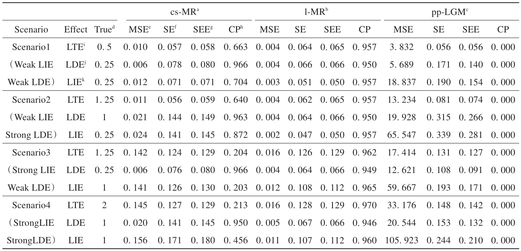
Assumption 4 LetAndenote an exposure variable at time pointn,Yman outcome variable at time pointm,andγnmthe causal effect ofAnonYm(0 ≤n≤m≤k), thenγnk= 0 forn

Assumption 5 LetGAdenote a genetic variable,Anan exposure variable at time pointn, andBna mediator variable at time pointn.Assume thatGAaffects {A0,…,Ak} only throughA0, its total genetic effect onAndepends onn, and the causal effect ofAnonBndo not depend onn.Specifically, letαndenote the direct effect ofGAonAn,αnmthe effect ofAnonAm, andβnmthe effect ofAnonBm(0 ≤n≤m≤k).Assume thatα0≠0,αn= 0 for 1 ≤n≤k, andαnm≠1 andβnn=βmmfor 0 ≤n≤m≤k.

Assumptions 1-3 specify parametric conditions for deriving the average causal effect in the traditional MR method.The newly proposed Assumption 4 is reasonable since we can expect that the effects of exposures and mediators on the final outcome satisfy the Markov property.Assumption 5 can be explained as follows.Since the genetic effects are congenital,GAhas no direct effects onA1,…,AkgiveA0.Since we assume that the causal effects are time varying,αnmshould not be 1.For example,A0andA1can be expressed asA0=γ0+α0GA+ε0andA1=γ1+α01A0+ε1=γ1+α01γ0+α01α0GA+α01ε0+ε1, respectively, so that the effects ofGAonA0andA1areα0andα01α0, respectively.Therefore, the genetic effects are time varying if and only ifα01≠1.Furthermore, it is reasonable to assume that the effect of the exposure on the mediator at the same time point is time independent(βnnis free ofn).

We have the following identifiability results:

Theorem 1 Under the longitudinal mediation model (1) and Assumptions 1-5, LMEs can be expressed asμLTE=γa1+γb1(βa00βb01+βa01+βa11),μLDE=γa1, andμLIE=γb1)

(βa00βb01+βa01+βa11.

The proof of Theorem 1 is postponed to Appendix A.1 in Supplementary Material.

1.5 Statistical inference of LMEs and its large sample properties

From now on, we focus on the model depicted in Fig.1(b).We present an estimation algorithm for LMEs and some associated large sample properties including consistency and asymptotic normality.Our method is based on MVMR and univariable MR.

According to Theorem 1, we only need to estimateβa00,βb01,βa01,βa11,γa1,γb1, which can be determined byθ1,…,θ8depicted in Fig.2 and Fig.3:

Fig.2 Two models extracted from the proposed model shown in Fig.1(b)

Fig.3 Models extracted from the proposed model shown in Fig.1(b)

where the causal effectsθ1,θ2,θ6andθ7can be estimated using MVMR, the causal effectsθ3,θ4,θ5,θ8can be estimated using univariable MR.

Plugging the above expressions into the formulas in Theorem 1, we have (refer to Appendix A.2 in Supplementary Material for a proof)

We propose to estimateθ1,…,θ8using MVMR and univarible MR.Specifically, applying MVMR (Burgess et al.,2015) to the models depicted in Fig.2(a) and Fig.2(b), we can obtain consistent estimates of (θ1,θ2) (denoted by (θ̂1,θ̂2)) and (θ6,θ7)(denoted by (θ̂6,θ̂7)), respectively; Applying the univariable MR method (Grover et al.,2017), we can obtain consistent estimates ofθ3,θ4,θ5, andθ8based on models depicted in Fig.3, which are denoted byθ̂3,θ̂4,θ̂5, andθ̂8, respectively.

Denote Θ =(θ1,θ2,θ3,θ4,θ5,θ6,θ7,θ8)' and Θ̂ =(θ̂1,θ̂2,θ̂3,θ̂4,θ̂5,θ̂6,θ̂7,θ̂8)'.LetLT(Θ̂),LD(Θ̂), andLI(Θ̂) be the resulting estimators of the LMEsμLTE,μLDE, andμLIE.

Theorem 2 Under the model depicted in Fig.1(b) and Assumptions 1-5, we have the following large sample properties:

According to the theorem above, we can derive the confidence intervals of LMEs.

2 Simulation studies

2.1 Considered methods

We considered three methods in our simulation studies.The first method is our proposed method, which is termed l-MR since it is a Mendelian randomization method designed for longitudinal data.The second method is the traditional Mendelian randomization method designed for cross-sectional studies (termed cs-MR) (Burgess et al.,2015).The third method is the parallel process latent growth curve modeling (pp-LGM) (Cheong et al.,2003)developed in the framework of structural equation modeling (SEM), which is specifically tailored for longitudinal mediation analysis without using IVs.

2.2 Data generation models

Data were generated according to the following linear models:

whereGA,GAB,GBwere independent and identically distributed from the Bernoulli distribution with trial number 2 and successful rate 0.3, andU1,U2,U3,εA0,εB0,εA1,εB1,εA2,εB2, andεYwere standard normally distributed.HereGA,GAB, andGBmeasure additive genetic patterns of three biallelic genetic variants with a common minor allele frequency of 0.3, which serve as instrumental variants forA,B, and (A,B), respectively.U1,U2, andU3quantify different confounders in the associations between the exposure, mediator, and outcome.

In the next three subsections, we consider three situations: the first with Assumption 4 and Assumption 5 satisfied (Section 2.3), the second with Assumption 4 or Assumption 5 violated (Section 2.4), the last with selection bias of IVs (Section 2.5).In all situations,αa01= 0.8,αa12= 0.75,βa00= 0.26,βb01= 0.8,βa01= 0.121,βa11= 0.26,βb12= 1,βa12= 0.151 andβa22= 0.26.For each of the parameter combinations considered in the next three subsections, the simulation results reported in the next subsection were based on 1 000 data sets of size 3 000.

2.3 Assumption 4 and Assumption 5 satisfied

We considered various combinations ofγa2andγb2: (γa2= 1,γb2= 1), (γa2= 1,γb2= 0.25), (γa2= 0.25,γb2=1), and (γa2= 0.25,γb2= 0.25), corresponding to four causal effect scenarios: (strong LDE, strong LIE), (strong LDE, weak LIE), (weak LDE, strong LIE), (weak LDE, weak LIE).The other parameters were fixed:αg0= 0.9,αgab= 0.9,βg0= 0.9,βgab= 0.9,αg1= 0,βg1= 0,αg2= 0,βg2= 0,γa0= 0,γb0= 0,γa1= 0, andγb1= 0.All of these scenarios have strong IV effects indicated byαg0= 0.9,αg0= 0.9,βg0= 0.9, andβgab= 0.9.

We also considered various combinations ofαg0,αgab,βg0, andβgab: (αg0=βg0= 0.9,αgab=βgab= 0.9), (αg0=βg0= 0.9,αgab=βgab= 0.3), (αg0=βg0= 0.3,αgab=βgab= 0.9), and (αg0=βg0= 0.3,αgab=βgab= 0.3), corresponding to four IV effect scenarios: (strong single genetic effect, strong pleiotropic genetic effect (Burgess et al.,2015)), (strong single genetic effect, weak pleiotropic genetic effect), (weak single genetic effect, strong pleiotropic genetic effect), (weak single genetic effect, weak pleiotropic genetic effect).Here single genetic effect refers to the effect of genetic variants without pleiotropy and pleiotropic genetic effect refers to the effect of genetic variants with pleiotropy.All of the above scenarios have weak LDE and strong LIE indicated byγa2= 0.25 andγb2= 1.

Table1 shows mean estimates, mean square errors (MSE), mean standard errors (SE), coverage probabilities(CP), and standard error of the estimates of these effects (SEE).

In all of the four scenarios for various causal effect combinations, the l-MR method outperforms the other methods in estimating LMEs.Overall, the l-MR method has very minor estimation biases, SEs close to SEEs,and coverage probabilities close to the nominal level 95%.Since the cs-LGM method assumes that genetic effects are constant but the true values are time varying, it is not surprising that the estimation biases were quite large and the coverage probabilities were low.Due to the definition difference, the estimation results of the pp-LGM method were also poor, with the largest estimation biases and the lowest coverage probabilities among the three considered methods.

Simulation results for the four IV-effect combinations are reported in Table2.The estimation efficiency of the l-MR method appeared to be largely affected by pleiotropic genetic variants.To be specific, strong pleiotropic genetic variants favored the estimation of LMEs indicated by much smaller SEs and well controlled CPs.In the weak-IV situation, however, the l-MR method had a poorer performance indicated by much larger SEEs and slightly inflated CPs.In addition, cs-MR and pp-LGM perform much poorer than l-MR in terms of estimation biases and CPs in all of the four scenarios.

2.4 Assumption 4 or Assumption 5 violated

The l-MR method is based on Assumption 4 and Assumption 5, but these assumptions could be violated inreal world.In order to investigate the robustness of l-MR, we considered three scenarios with either Assumption 4 or Assumption 5 being violated: (Assumption 4 violated, Assumption 5 satisfied), (Assumption 4 satisfied, Assumption 5 violated), and (Assumption 4 violated, Assumption 5 violated).

Only Assumption 4 violated.We variedγa0=γb0andγa1=γb1from 0 to 0.25.Here 0.25 was the critical value such that the causal effects ofA0,B0,A1, andB1were smaller than or equal to those ofA2andB2.The estimation biases of l-MR and cs-MR are depicted in Fig.4, the coverage probabilities of 95% confidence intervals of l-MR are depicted in Fig.5, and the estimation results of l-MR are summarized in Table3.As expected, cs-MR and l-MR had the same estimation biases for LDE, which were minor overall.As for LTE and LIE, cs-MR had much larger biases for LTE and LIE, and the biases of both methods were gradually increasing withγa0andγa1.The CPs were decreasing withγa0.To be specific, as for LTE, the CP ≥88.7% forγa0< 0.125 ; as for LDE, the CP ≥86.9% forγa0< 0.062 5; as for LIE, the CP ≥87.0% forγa0< 0.062 5.The results suggest that l-MR is somewhat robust to the violation of Assumption 4.

Fig.4 Estimation biases under model (3) with Assumption 4 violated.Four effects quantifying departure from Assumption 4(i.e., γa0, γa1, γb0, and γb1) were assumed to be the same and ranged from 0 to 0.25.The three subfigures show the estimation biases of cs-MR (the traditional Mendelian randomization designed for cross-sectional data) and l-MR(our proposed method designed for longitudinal data) for LTE, LDE, and LIE, respectively.

Fig.5 Coverage probabilities (CPs) of 95% CIs of causal effects LTE, LDE, and LIE by l-MR with Assumption 4 violated.Refer to the caption of Fig.4 for simulation settings.The red dashed line represents the nominal level 0.95.

Only Assumption 5 violated.It is natural to assume that the effect ofGAonA1does not exceed that ofGAonA0, i.e.,αg1+αg0αa01≤αg0and Assumption 5 holds whenαg1+αg0αa01=αg0.Consequently, we variedαg1from 0 to (αg0-αg0αa01).Similarly, we assume that the effect ofGAonA2does not exceed that ofGAonA0.Therefore,we variedαg2from 0 to (αg0-αg0αa12).The estimation results of l-MR are summarized in Appendix C Table S.2(Supplementary Material), the estimation biases of l-MR and cs-MR are depicted in Appendix B Figure S.1(Supplementary Material), and the coverage probabilities of 95% confidence intervals of l-MR are depicted in Appendix B Figure S.2 (Supplementary Material).The estimation biases of LTEs and LIEs by cs-MR were evidently decreasing withαg1.This is reasonable since the violation of Assumption 5 is decreasing withαg1forαg1≤(αg0-αg0αa01) andαg2forαg2≤(αg0-αg0αa12).On the other hand, the biases of l-MR were very minor for allαg1andαg2, demonstrating that l-MR is robust to the violation to Assumption 5 to some extent.

Both Assumption 4 and Assumption 5 violated.We variedγa0=γb0=γa1=γb1from 0 toγa2,αg1=βg1from 0 to (αg0-αg0αa01), andαg2=βg2from 0 to (αg0-αg0αa12).The estimation biases of l-MR and cs-MR are depicted in Appendix B Figure S.3 (Supplementary Material), the coverage probabilities of 95% confidence intervals of l-MR are depicted in Appendix B Figure S.4 (Supplementary Material), and the estimation results of l-MR are summarized in Appendix C Table S.3 (Supplementary Material).Similar to the simulation results with only Assumption 5 violated, the estimation biases of LTEs and LIEs by cs-MR were evidently decreasing withαg1, and approximately equal to the estimation bias with l-MR whenαg1=αg0-αg0αa01, as expected.Additionally, the biases of LDEs by l-MR and cs-MR were simultaneously increasing withαg1.Generally speaking, l-MR is doubly robust to the violation of Assumption 4 and Assumption 5.

2.5 Selection bias of instrumental variables

Mendelian randomization analysis, on which l-MR method is based, suffers from bias caused by selecting instrumental variables.In order to investigate the influence of selection bias on l-MR, we considered six true ge-netic instruments scenarios: (two strong genetic instruments related to the exposure, a strong pleiotropic genetic instrument, a strong genetic instrument related to the mediator), (a strong and a weak genetic genetic instruments related to the exposure, a strong pleiotropic genetic instrument, a strong genetic instrument related to the mediator), (two strong pleiotropic genetic instruments, a strong genetic instrument related to the exposure,a strong genetic instrument related to the mediator), (a strong and a weak pleiotropic genetic instruments, a strong genetic instrument related to the exposure,a strong genetic instrument related to the mediator), (two strong genetic instruments related to the mediator, a strong pleiotropic genetic instrument, a strong genetic instrument related to the exposure), and (a strong and a weak genetic genetic instruments related to the mediator, a strong pleiotropic genetic instrument, a strong genetic instrument related to the exposure).All of these scenarios have strong IV effects indicated byαg0= 0.9,αgab= 0.9,βg0= 0.9, andβgab= 0.9, weak LDE and strong LIE indicated byγa2= 0.25 andγb2= 1.

Simulation results for the six true genetic instruments scenarios are reported in Appendix C Table S.4(Supplementary Material).The estimation efficiencies of l-MR, cs-MR, and pp-LGM are close to their respective performance in the situation where the true genetic instruments are a strong genetic instrument related to the exposure, a strong pleiotropic genetic instrument, and a strong genetic instrument related to the mediator (i.e.Scenario 3 in Table 1).The selection bias has minor impact on l-MR in the simulation situations.

Table 1 Estimation results of simulation

Table 2 Estimation results for simulating the effects of weak instrumental variables

Table 3 Performance of l-MR in the case of violating Assumption 4

3 Discussion

In observational studies, instrumental variables are widely used to control estimation biases of causal effects due to confounding and reverse causation.Longitudinal data can be used to capture the mediator process more finely, and lifetime mediation effects have been defined to reflect the nature of such process.However, there is no instrumental variable method, including Mendelian randomization, specially tailored for longitudinal mediation analysis in the literature.

In this paper, we considered a longitudinal mediation model with time-varying genetic effects.It has been shown that the traditional Mendelian randomization method cannot consistently estimate LMEs under such model.Under several reasonable assumptions, we first established the identifiability of lifetime mediation effects, then developed a new Mendelian-randomization based method to estimate longitudinal mediation effect,which is consistent in the presence of time-varying genetic effects.Simulation studies were conducted to demonstrate the desired performance of our proposed method.The results showed that the proposed method generally outperform existing methods in estimating lifetime mediation effects in the presence of time-varying genetic effects.Sensitivity analysis studies showed that the proposed method is much more robust to the violation of two assumptions for the validity of Mendelian randomization, compared with the traditional longitudinal mediation analysis methods.

Our method still has several limitations, part of which are shared by the traditional MR methods (Smith et al.,2004).For example, the method could suffer from the weak instrument bias.Second, our proposed method estimates time-varying parameters sequentially, which becomes quite complex if too many time points are involved.It deserves further investigation to develop more suitable method, such as latent growth curve modeling method (Soest et al.,2011) in such situation.

4 Supplementary material

Supplementary material is available at https://github.com/SherryJ-lab/Supplementary-Material.