Optimal confrontation position selecting games model and its application to one-on-one air combat

Zekun Dun , Genjiu Xu ,b,*, Xin Liu , Jiyun M , Liying Wng

a School of Mathematics and Statistics, Northwestern Polytechnical University, Xi'an 710072, China

b International Joint Research Center on Operations Research, Optimization and Artificial Intelligence, Xi'an 710129, China

c AVIC Xi’an Aeronautics Computing Technique Research Institute, Xi'an 710065, China

d Unmanned System Research Institute, Northwestern Polytechnical University, Xi'an 710072, China

Keywords: Unmanned aerial vehicles (UAVs)Air combat Continuous strategy space Mixed strategy Nash equilibrium

ABSTRACT In the air combat process, confrontation position is the critical factor to determine the confrontation situation, attack effect and escape probability of UAVs.Therefore, selecting the optimal confrontation position becomes the primary goal of maneuver decision-making.By taking the position as the UAV's maneuver strategy, this paper constructs the optimal confrontation position selecting games (OCPSGs)model.In the OCPSGs model, the payoff function of each UAV is defined by the difference between the comprehensive advantages of both sides, and the strategy space of each UAV at every step is defined by its accessible space determined by the maneuverability.Then we design the limit approximation of mixed strategy Nash equilibrium (LAMSNQ) algorithm, which provides a method to determine the optimal probability distribution of positions in the strategy space.In the simulation phase, we assume the motions on three directions are independent and the strategy space is a cuboid to simplify the model.Several simulations are performed to verify the feasibility, effectiveness and stability of the algorithm.© 2023 China Ordnance Society.Publishing services by Elsevier B.V.on behalf of KeAi Communications

1.Introduction

With the development of technology,Unmanned Aerial Vehicles(UAVs)have come in a wide variety of applications and have played an indispensable role in modern air combat.The UAV combat is also emerging as an important research issue in the modern warfare[1].Generally, decisions of UAVs in the air combat mainly include tactical decisions [2,3] and maneuver decisions [4].The Tactical decision is a kind of exogenous decision focusing on the offensive and defensive behaviors similar to the fire attack, while the maneuver decision can be regarded as an endogenous decision focusing on taking advantage in the confrontation situation through controlling the maneuvers of UAVs.In this paper, we mainly study on the latter.In the maneuver decision problem, the confrontation relationship between UAVs is regarded as a pursuit and evasion scenario that UAVs aim to constantly take the initiative in the battlefield by formulating the optimal flight position.Therefore,the key to this problem is how the aircraft should select the best maneuver strategy.

Common research methods used in decision-making for air combat maneuvers include the optimization theory method[5-8],the expert system method [9-11] and the reinforcement learning method [12-15].

The optimization theory method uses genetic algorithm,Bayesian preference and statistical theory to make the best maneuver decision from a finite and discrete strategy space through optimizing the objective function of the aircraft.However,the realtime performance of numerous optimization algorithms is low in large-scale problems.The expert system method uses artificial intelligence technology and computer technology to summarize a rule base, where UAVs can find the best strategies for different battle scenarios.Nevertheless,it is difficult and time-consuming to get a complete rule base that can cover the diverse combat situations.The reinforcement learning method, continually learns strategies to maximize revenues or achieve specific goals through the interaction between agents and the environment.This approach has been used extensively in air combat decision-making,while it is not interpretable and stable.

In the combat process, the attack effect and the interception capacity of UAVs are mainly linked to the situation of UAVs.Therefore, how should the aircraft make the best maneuver decision without knowing the opponent's plan for maintaining the dominant situation? [16] Obviously, this is a game process.Game theory is a type of mathematical method for studying the problem of interactive optimization of decision-making[17].In Comparison with the methods mentioned above, the most important point of game theory is to take the uncertainty of the decision-making of opponents into account.From this point of view, the approach of game theory is more suited to the study of the optimal interactive maneuver decision of UAVs.

Matrix game is a basic and useful tool to study the maneuver decision problem for UAVs.In 1987, Austin et al.[18] pioneer the framework of matrix game model to analyze the optimal interactive maneuver decision for air-to-air combat.Subsequently, many researchers [19-22] use matrix games to model the maneuver decision-making process of air combat.This method can only be used to solve the optimal decision in the current situation,but the result is not necessarily the optimal decision in the whole process of air combat.For the farsightedness of decision, Virtanen et al.[23,24] combine the influence diagram method with the game method, proposing the multistage influence diagram game model for modeling the maneuver decisions of aircrafts in one-on-one air combat.Based on this model,some scholars[25,26]expand the air combat scenario from one-on-one to multi-UAVs.Compared with other maneuver decision models based on game approach, this method can reflect the preference of the pilot and have good performance under uncertain information, but it is difficult to obtain reliable prior knowledge[27].

In all above maneuver decision methods, the strategy space of the UAV is generally discretized into given finite actions according to the basic air combat maneuver divided by NASA [18,28], where UAV's strategy is composed of dynamic maneuver variables,such as overload and rolling angle.However, the finite strategy space will limit the flexibility of UAV's maneuver and lead to a gap between the simulation environment and the actual environment.

In essence, the confrontation situation is to find the best position, and the position is observable compared with the maneuver actions.Additionally,the strategy space should be continued since the ever-changing and dynamic character of the battle situation.Therefore, we use the position as a maneuver strategy for UAVs in this paper.Based on the strategy space composed of the positions that the UAV can reach,we introduce a new optimal confrontation position selecting games (OCPSGs) model.In order to solve this game model with continuous strategy space,we propose the limit approximation of mixed strategy Nash equilibrium (LAMSNQ)algorithm.

Situation assessment take a virtual role in the decision-making process.Huang et al.[6] define a maneuver decision factor to evaluate the situation, which is composed of angle factor, height factor,distance factor and velocity factor.Austin et al.[28]and Park et al.[29] define the scoring function to evaluate the situation,which are all composed of distance factor,angle factor and velocity factor,but the former has one more terrain factor.¨Ozpala et al.[30]and Chen et al.[31] define the total superiority and the index of situation, respectively, to evaluate the air combat situation, which are also includes distance, angle and speed.In OCPSGs model, we assume the confrontation situation is affected by the relative distance,angles between speed vector and line of sight(lag angle and lead angle), and speeds of UAVs, which are all determined by the positions of both sides.Based on these factors we define the comprehensive advantage function to evaluate the confrontation situation.The payoff function is defined as the difference between the comprehensive advantages of both sides.It leads to a twoperson zero-sum game model, where the strategy is the UAV's position.The strategy space of the UAV at every moment is the accessible space determined by maneuverability of the UAV.In the decision-making process,the UAV is not able to predict the precise position of the opponent at the next stage.Based on this uncertainty, we can find an optimal probability distribution for all positions in the accessible space to maximize the expected utility of the UAV.Such a probability distribution is actual a mixed strategy in the strategy space.Consequently, the OCPSGs model is transformed into the problem of solving the mixed strategy Nash equilibrium(MSNE).

Generally,linear programming and intelligent search algorithm can be used to solve the MSNE of finite and discrete strategy spaces.However, these two methods are no longer suitable for nonlinear objective function and continuous strategy space scenarios.For that reason, the LAMSNQ algorithm is based on integrating the nonlinear objective function.Firstly,we divide the strategy space of each step of the UAV into several small spaces of the same size,and then calculate the optimal probability distribution on the small spaces based on maximizing the expected utility.This optimal probability distribution is the approximate mixed strategy Nash equilibrium (AMSNE) of the OCPSGs model.Then, we select the center of the small space corresponding to the maximum probability of the AMSNE as the optimal confrontation position of the UAV.Finally, we simulate several experiments under different conditions and confrontation scenarios, and the results verify the feasibility, effectiveness and stability of the algorithm.

The remainder of this paper is organized as follows.Section 2 introduces the problem description and related notations.Section 3 proposes the OCPSGs model and designs the LAMSNQ algorithm.Section 4 conducts simulation analysis.Section 5 concludes the paper.

2.Problem formulation and preliminaries

2.1.Problem description

Let us consider an one-on-one confrontation scenario in a threedimensional space,and the schematic diagram of UAVs is displayed in Fig.1.We assume that each UAV knows the position and speed of another side of the current moment and one side will launch an attack once another side enters its attack range.

Fig.1.Geometry relationship of UAVs in the 3-dimensional space.

There are two UAVs in the maneuver decision model.Specifically,the confrontation sides are labeled as the red aircraft and the blue aircraft,which are denoted byrandb,respectively.Each UAV is fully described by its location and velocity.P denotes the position vector and v denotes the speed vector.The maneuver decision process ofrandbincludes modeling the confrontation situation assessment, constructing the OCPSGs model to describe the interactive process of decision-making and solving the proposed game model.

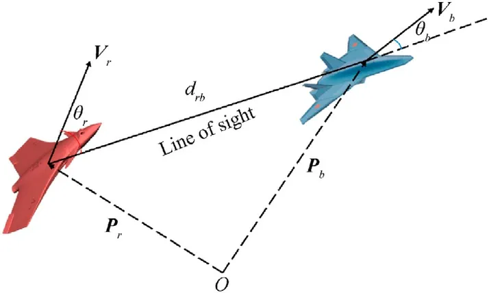
Fig.2.Diagram of variable relationship.

2.2.Kinematics characterization of the UAV and related notations

In this paper, we regard UAV as a point mass rather than a specific model in reality.For the red force, the position vector and speed vector are given by

wherexrandyrare horizontal coordinates,zris the altitude ofr,andis the derivative of the position vector ofrwith respect to time.

For the blue, the position vector and the speed vector can be expressed as

Letdrbdenote the distance betweenrandbon the line of sight,that is

Considering that the persistence of maneuvers will cause delays in the implementation of strategies, the aircraft needs to make decisions step by step according to the time interval denoted by Δt,which reflects the dynamic nature of the strategy.Accordingly,we propose the time delay constraint to describe this process,that is,rmakes a decision at timetandbreacts at timet+ 1,namely,.

At timet, the speed vector of the aircraft is given by

And the speed of the aircraft is given by

For reference,a graphical representation of θrand θbcan be seen in Fig.2.The angles are shown from the point of view of the red.We denote by θrthe angle between Pb-Prand vr,named as lag angle,and θbfor the angle between Pb-Prand vb,named as lead angle.At timet, lag angle and lead angle are given by

By analyzing the equations of the relative distance, angle between the speed vector and line of sight,and speed of the aircraft,it can be found that they are only related to the position vectors of both sides.Therefore, we will utilize this character to design the decision-making model of air combat.

2.3.Assessment of confrontation situation

In this subsection, we define a comprehensive advantage function of UAV in the basis of relative distance, angle between the speed vector and line of sight, and speed to evaluate the current situation and guide the maneuver strategy at the next moment.

2.3.1.Distanceadvantagefunction

Distance advantage is not only related to the distance between both sides but also related to the attack range of the weapons that carried by UAV [31].In the confrontation process, the attack probability of weapons will be reduced if the distance between the two sides is too far,while there will be security problems if the distance is too close.Therefore,there exists an optimal distance to maximize the attack probability on the premise of UAV's security.

For the red, the distance advantage function [32] can be configured as

whereKris a coefficient used to denote by the maneuver ability of the red,Dris the optimal attack distance.For the aircraft, a higherKrvalue indicates better maneuverability of the UAV.The value of distance advantage is in the range of(0,1],with the maximum of 1 whendrbis equal toDr.

2.3.2.Angleadvantagefunction

Park et al.[29] propose two necessary conditions for the aircraft's air superiority, that is, it has to be located at the rear of the opponent and heading for it.This indicates that the angle has a critical impact on the superiority of the combat situation.

It can be seen from Fig.2,if θr=θb=0,the red pursues the blue and the angle advantage of the red is the maximum.On the contrary, θr=θb=π means the red is pursued by the blue, and the angle advantage of the red is zero.If θr=0 and θb= π, the angle advantage of both sides are equal, namely, the two sides are wellmatched.Based on the above analysis, we define the angle advantage function [18] of the red as follows:

and the angle advantage function of the blue is defined by

Therefore, the angle advantage would have values between 0 and 1.For the red,Frawill be 1 when it is on the tail ofb, and 0 whenbis on the tail ofr.

2.3.3.Speedadvantagefunction

In addition to distance and angle, speed is also a vital factor in the combat situation.A higher speed will make the aircraft have more initiative, and make it easier to approach to or escape from the opponent.We denote by vrand vbthe scalar speed of the red and the blue respectively, which are given by

We denote by vr*the ideal speed of the red,

where vmaxis the maximum scalar speed of the UAV.For the red,when the distance between UAVs is much farther than the optimal attack distanceDr,the red should accelerate to shorten the distance with the opponent,namely,the ideal speed tends to vmax.Whendrbis equal toDr, vr*is equal to vbin order to keep the distance advantage.For the other cases, vr*is between vband vmax, and the actual value of vr*is determined by the distancedrb.The ideal speed of the blue vb*can be obtained in the same way.Simultaneously,the ideal speed is always larger than the speed of the opponent to keep the relative superiority.

For the red,the speed advantage function is defined as the ratio of actual speed to ideal speed, which is given by

In this equation, |vr-vr*|/vr*depicts the deviation degree between the actual speed and the ideal speed of the red.The smaller deviation means the larger speed advantage, that is, the UAV can reach the optimal attack distance faster and form the favorable attack conditions in shorter time.Similarly,we can define the speed advantage of the blue in the same way.

2.3.4.Comprehensiveadvantagefunction

The comprehensive advantage should be determined by the above factors.In this paper, we apply the method of convex combination of the factors [6,15,30,31] to describe the comprehensive advantage function.

Combining distance advantage, angle advantage and speed advantage, we define

to evaluate the real-time comprehensive advantage function of the red,and the comprehensive advantage function of the blue is

where ω1，ω2and ω3are weight coefficients, representing the importance of the corresponding advantage factors, 0 ≤ω1，ω2，ω3≤1 and ω1+ω2+ω3= 1.

2.4.Mixed strategy Nash equilibrium on continuous strategy space

In this paper,UAV's strategy is on the basis of mixed strategy of the game model.Consequently, we introduce some relative descriptions about the mixed strategy and mixed strategy Nash equilibrium in this subsection.

(Strategic Form Game)A strategic form 2-person game Γ is a tuple 〈｛r，b｝，S=Sr×Sb，｛Ui｝i=r，b〉， where

(1)ris the red aircraft andbis the blue aircraft;

(2)SrandSbare the strategy spaces ofrandbrespectively;

(3)Ur:Sr×Sb→R andUb:Sr×Sb→R are payoff functions of the red and the blue.

(Zero-Sum Game)A two-person zero-sum game is a tuple〈｛r，b｝，S=Sr×Sb，｛Ui｝i=r，b〉， whereSrandSbare the strategy sets of the players,andUiis a function such thatUi:Sr×Sb→R andUb（sr，sb） = -Ur（sr，sb）, for any strategy pair （sr，sb）∈Sr×Sb.

(Mixed Strategy on Continuous Strategy Space)On continuous strategy space,a mixed strategy forrisfand a mixed strategy forbisg, so thatf:Sr→［0，1］ is the probability density function ofr’s strategy andg:Sb→［0，1］ is the probability density function ofb’s strategy.The probability density functionsf（·）andg（·）satisfy the following two conditions:

(1)f（sr）≥0 andg（sb）≥0, for allsr∈Srandsb∈Sb;

(Expected Payoff on Continuous Strategy Space)Let the probability density functions of the red and the blue aref（sr） andg（sb）,respectively,Ur（sr，sb）andUb（sr，sb）are payoffs ofrandbwith the strategy pair（sr，sb）,wheresr∈Srandsb∈Sb.Then,the expected payoff of the red on continuous strategy space is given by

The expected payoff of the blue on continuous strategy space is given by

If Γ is a zero-sum game,we have

(Mixed Strategy Nash Equilibrium)Mixed strategy Nash equilibrium is a relatively stable state when players have conflicts of interest in the rational situation,and no player would unilaterally change this state.A mixed strategy pair （f*（sr），g*（sb）） is a mixed strategy Nash equilibrium for a 2-person game, if for allf（sr） andg（sb）, it holds that

If Γ is a zero-sum game, we can obtain another definition of mixed strategy Nash equilibrium from Eqs.(18)-(20).A mixed strategy pair（f*（sr），g*（sb））is a mixed strategy Nash equilibrium if and only if for allf（sr） andg（sb）, it holds that

3.OCPSGs model

In this section, we propose the optimal confrontation position selecting games model to describe the dynamic interaction process and make the optimal position decision for the UAV.In the confrontation process,the pure strategy is the position of the UAV,and the strategy space is composed of the positions that an UAV can reach determined by the maneuverability and time interval.

3.1.Strategy set and payoff function of the game

In this subsection, we construct the game model of air combat,and analyze the strategy set and payoff functions.

(1) Player set:N= ｛r，b｝;

(2) Strategy set:S=｛Sr，Sb｝, where

Ωrand Ωbare the accessible spaces ofrandbat the next step,respectively, which are determined by the kinematic limitations,the maneuverability and the time interval.Specifically,the strategy of UAViat timetisand

(3) Payoff functions:Ur（sr，sb）andUb（sr，sb）are payoff functions of the red and blue with the strategy pair（sr，sb）,respectively,which are denoted by

wheresr∈Sr，sb∈Sb.Obviously,

Then we analyze the payoff functions at timet+ 1.The distance advantage function ofrat timet+1 is given by

The angle advantage function ofrat timet+1 is given by

The speed advantage function ofrat timet+1 is given by

where

Accordingly,we can get the comprehensive advantage function ofrat timet+ 1, which is given by

Similarly, the comprehensive advantage function ofbcan be expressed as

The payoff functions ofrandbat timet+1 are defined by

Considering the time delay constraint in subsection 2.2, the position of the blue at timet+1 is determined that we don't need to consider its strategy probability density function at timet.Under this constraint, the expected payoff ofrat timet+1 according to Eq.(16) can be simplified as

According to Eq.(19),the equilibrium strategy ofrat timetis the probability density function maximizing the expected payoff,which is given by

So far,we have analyzed the strategy set and payoff functions for this game model.The optimal strategy of the UAV at timetis to select the optimal position at timet+ 1, which is relative to the mixed strategy Nash equilibrium of this game model.In the next subsection,we will propose an algorithm to solve the approximate equilibrium.

3.2.LAMSNQ algorithm

Inspired by paper [33], we design the LAMSNQ algorithm to obtain the mixed strategy Nash equilibrium of the OCPSGs model,and use the equilibrium solution to determine the optimal strategy.The algorithm steps for UAVrat timetare illustrated as follows.

Fig.3.Decision-making framework for UAVs.

Step 1: At first, we need to determine the strategy space ofr.According to the kinematic limitations and time interval, we can calculate the accessible space ofrat the next step, which are denoted by Ωrreferring to the strategy space ofr.

Step 2: We divide the strategy space ΩrintoMequally small spaces denoted by Ωri，i= 1，2，…，M.

Step 3: After dividing the strategy space, we need to find the optimal probability distributions on the small spaces Ωri.According to Eq.(35), it holds that the determination of the optimal probability distribution is based on maximizing the expected payoff.Consequently, we can transform this problem into the following optimization problem, which is given by

prirepresents the probability ofrreaching theith small space Ωri.Rris the expected payoff ofr.By solving the programming problem in Eq.(36), we can derive the optimal probability distributionp*=.

Step 4: In the case of continuous strategy space, we fit the optimal probability density functionof strategy space by the linear regression of （ξr1，ξr2，…，ξrM） and.ξriis the center position ofith small space.

we can obtain the maximum expected payoff Er on the continuous strategy space.Substituting p* into the objective function of Eq.(36), we have the maximum expected payoff Rr* on the discrete strategy space.We set ε = 10-3, if the termination conditionis satisfied,is the mixed strategy Nash equilibrium ofr, so we can use the discrete probability distributionp*to approximate the probability of a strategy on the continuous space.Otherwise, the strategy space Ωrneeds to be subdivided into 2Mequal parts,3Mequal parts…and we need to redefine the strategy space and repeat the above steps after that.

Step 6: If the termination condition is satisfied, we can derive the optimal strategy ofr, that is, the position with the maximum probability.The coordinate of the optimal position is the center of the small space with the maximum probability, which is denoted by, where

Step 7:At each step in the combat process,rupdates its position according to the optimal position obtained in step 6 and determines whether the distance between two sides is less than or equal to its own optimal attack distance, namely,drb≤Dr.If satisfied, the confrontation ends, and the winning probabilities of both sides are defined as Softmax functions, which are given by

whereFrandFbare terminal comprehensive advantage functions of the red and the blue respectively, and the side with the higher winning probability wins the air combat.To illustrate the process of the algorithm, the flow chart of LAMSNQ algorithm is displayed in Fig.4.

4.Simulation and analysis

4.1.Model reduction

To simplify the analysis,we suppose that the motions of UAVs onX-axis,Y-axis andZ-axis are independent of each other.Consequently, the accessible space of the aircraft within a time interval forms a cuboid that is determined by its upper and lower limit of the motion in the direction of three axes.This cuboid is the strategy space in which the aircraft will select the optimal position,and the position of the UAV at the next step is the optimal position in the cuboid.The strategy spaces of both sides are defined as follows.

Then we analyze the strategy space at timet.The strategy space at timetis the accessible zone of the UAV, which is limited by the maximum direction acceleration and minimum direction acceleration.Given the position and speed of the UAV at timet, we can describe its accessible space onX-axis.Fori∈｛r，b｝, we have

Under the assumption of motion independence, the direction probability density functions on the strategy space at timet+1 are denoted byTherefore, the probability density function ofrin Eq.(34) is denoted by

Accordingly, Eq.(34) can be further expressed as

Based on the above simplification process,we can transform the first five steps of the LAMSNQ algorithm into the following form.

Step 1: According to Eqs.(43) and (44), we can calculate the ranges of motion ofrin the direction of coordinate axes,which are denoted byrespectively.Then we can get a cuboidreferring to the strategy space ofr.

Step 2: We divide the strategy set on each coordinate axis ofrintoMequal intervals, and the strategy space is divided intoM3small cuboids.are the left endpoints on themth interval ofX-axis, thenth interval ofY-axis and thelth interval ofZaxis, respectively, which are defined by

With the increase ofM,the computational complexity increases exponentially.In order to decrease the computational complexity,we selectMpoints denoted by ｛ξ1， ξ2， …， ξM｝, where ξkis an abbreviation for ξk，k，k, for allk=1，2，…，M.We want to approximate the probability density function of the strategy space ofrby the probability distribution at these points solved in step 3.

Step 3: After dividing the strategy space, we need to find the optimal probability distributions in the direction of three coordinate axes of the points ｛ξ1，ξ2，…，ξM｝.Based on maximizing the expected payoff,we can define the following optimization problem.

Pxk，PykandPzkrepresent the probability ofrreaching thekth point onX-axis,Y-axis andZ-axis respectively.Rris the expected payoff ofr.By solving the programming problem in Eq.(48),we can derive the optimal probability distribution, where

Step 4:We fit the probability density function ofX-axisby linear regression of.Similarly,we can obtain the probability density functions ofY-axis andZ-axis,namely,.

Fig.4.The flow chart of LAMSNQ algorithm.

We can obtain the maximum expected payoffEron the continuous strategy space.SubstitutingP*into the objective function of Eq.(48), we have the maximum expected payoffR*on the discrete strategy space.We set ε = 10-3, if the termination conditionis satisfied,is the mixed strategy Nash equilibrium ofr, so we can use the discrete probability distributionP*to approximate the probability of a strategy on the continuous space.Otherwise,the strategy set in the direction of each coordinate axis needs to be subdivided into 2Mequal parts,3Mequal parts … and we need to redefine the strategy space and repeat the above steps after that.

Step 6: If the termination condition is satisfied, we can derive the optimal strategy ofr, that is, the position with the maximum probability on each axis.The coordinate of the optimal position is denoted bywhere

4.2.Numerical simulation and result analysis

4.2.1.Settingsofparameters

To verify the effectiveness of the OCPSGs model,simulations are performed in this section.We use Python to do all simulations and all experiments satisfy the time delay constraint.The winning probabilities of UAVs are defined in Eqs.(39) and (40).In order to simplify the simulation scene, we simulate the confrontation process in a two-dimensional plane.We use Python SciPy Optimizers to solve the nonlinear programming in Eq.(48).

The initial position and speed ofrare Pr=［5000，5000］and vr=［200，1］.The initial position and speed ofbare Pb=［1，1］and vb=［200，1］.The maximum scalar speed, maximum direction acceleration and minimum direction acceleration for each side are vmax=400 m/s，， anda= - 90 m/s2, respectively.Meanwhile, the optimal attack distances and the maneuver ability of UAVs areDr=Db=1500 m andKr=Kb=2,respectively,and the weight coefficients in Eqs.(14)and(15)are set as ω1=ω2=ω3=1/3.The simulation time interval is Δt= 0.5 s.

4.2.2.Bluekeepsconstantspeedflight

In this simulation,bkeeps the constant speed whileris equipped with the method designed in this paper.The trajectories of both sides are shown in Fig.5(a).The change trends of UAVs'comprehensive advantage are shown in Fig.5(b).

In the starting stage,bis on the tail ofr,so the blue is superior to the red.In the later stage,rperforms turn round and face tob,whilebis flying straightly.From Fig.5(b), we can see that the comprehensive advantage ofris constantly dominant the comprehensive advantage ofbafter Step 7.Obviously,rwin this game as its comprehensive advantage is bigger than that ofb, which is as expected.The red still wins under the initial condition that the angle advantage of the blue is dominant, which shows the effectiveness of our algorithm.

4.2.3.Bothsidesadoptthemethodinthepaper

In this section,the two UAVs are all equipped with the method proposed in this paper.The related figures are shown as follows.

From Fig.6 we can see that the two sides are far away from the initial state and both sides tend to approach each other.In the process of approaching,the tangent line of the trajectory at a point is approximated as the speed direction of the UAV.Therefore,it can be seen that the two gradually adjust the nose to aim at each other in the process of confrontation.Finally,the confrontation comes to an end when the distance between UAVs is less than or equal to the optimal attack distance of one party.

As can be seen from Fig.7(a),the distance between the two sides gradually decreases.At Step 23,the distance is less than the optimal attack distance and the confrontation ends.In Fig.7(b),the distance advantage is gradually increasing with the approaching of two sides.Given the initial values ofKandDare equal,so the distance advantage of both sides is also equal.

At the initial moment, we can calculate that θr= θb, but the angle advantage of the blue is larger.In Fig.8(a), as the confrontation continues, lead angle θbgradually increases and remains an obtuse angle while lag angle θrgradually decreases to an acute angle,indicating that the red keeps adjusting its speed direction to aim at the blue.In Fig.8(b), the angle advantage of the blue is no longer dominant after step 13, and the two sides are nearly in a head-to-head position after that, so the angle advantage of both sides is gradually tending to 0.5.The above analysis echoes the trajectories of both sides in Fig.6, that is, the red reverses its direction in the battle, and then the two sides gradually approach.

Fig.5.Confrontation trajectories and comprehensive change trend of UAVs: (a) Confrontation trajectories of UAVs; (b) Comprehensive advantage of UAVs.

Fig.6.Confrontation trajectories of the red and the blue.

As can be seen from Fig.9(a),before Step 13,the deviation index of the red|vr-vr*|/vr*gradually decreases and has been larger than|vb- vb*|/vb*.Hence, speed advantage of the red is smaller than that of the blue in Fig.9(b).From Step 14 to Step 17,we have |vb-vb*|/vb*＞|vr-vr*|/vr*.During the whole confrontation,the speeds of both sides are less than the maximum speed vmax.Combined with the formula of speed advantage and the change of distance between the two sides, we do the following analysis: Before Step 13, the red adjusts the angle to turn to face the blue behind itself,and the turn will inevitably cause a reduction in speed.According to the definition of speed advantage,the deviation between the red's speed and the ideal speed before Step 13 is larger than that of the blue,resulting in the speed advantage of the red is smaller than that of the blue.

Fig.10 shows the change trend of the comprehensive advantages of both sides in the confrontation process.Since the distance advantages of both sides are equal, so its effect on the comprehensive advantage can be neglected.Besides,the angle advantages of both sides are symmetrical.Accordingly, the main factor affecting the comprehensive advantage is the speed advantage.Through Figs.9(b)and Fig.10,we can see that the change trend of the comprehensive advantage is similar to the change trend of the speed advantage.At Step 23, the confrontation termination conditiondrb≤Dis satisfied, at this time the comprehensive advantage of the red is greater than that of the blue, so the winning probability of the red is higher and the red wins in the final.

4.2.4.Decisiontimeinterval,simulationtimeintervalanddivision intervalnumber

In LAMSNQ algorithm, we divide the strategy set on each coordinate axis intoNequal intervals, called the division interval number,to solve the approximate mixed strategy Nash equilibrium.Decision time interval refers to the physical time interval that triggers a simulation calculation in the system.Simulation time interval refers to the time interval we set in the simulation for the UAV to make a decision.

Fig.7.The change trend of UAV's distance and distance advantage value: (a) The distance between r and b; (b) The distance advantage of r and b.

Fig.8.The change trend of UAV's angle and angle advantage value: (a) The angle trend of r and b; (b) The angle advantage of r and b.

Fig.9.The change trend of speed deviation degree and speed advantage value: (a) The degree of deviation from ideal speed; (b) The speed advantage of r and b.

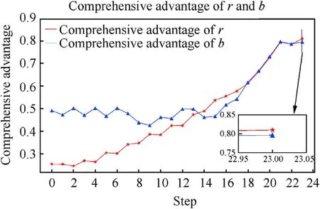
Fig.10.Changes in the comprehensive advantage of the red and the blue.

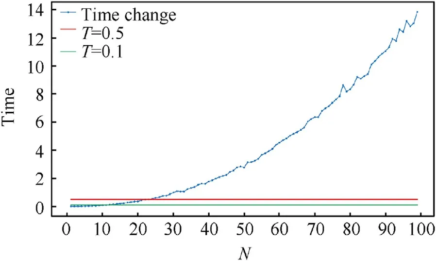
Fig.11.The relationship between division interval number and decision time.

Theoretically,we can take the time interval as small as possible to approximate continuous.However, the efficiency of the algorithm itself should be considered in practical application.From this point of view, we want to find the relationship between interval division number and decision time.

In Fig.11, lateral axis represents the division interval number and the vertical axis represents the decision time interval.The red line and green line represent the simulation time interval.It can be seen that the decision time interval increases with the increase ofN.When the simulation time interval is 0.5 s and 0.1 s, the correspondingNis about 23 and 10, respectively.

To ensure the simulation time interval is longer than the decision time interval, we know that the division interval number should not exceed 10 if the simulation time interval is 0.1 s,and the division interval number should not exceed 23 if the simulation time interval is 0.5 s.

4.2.5.Influenceofdivisionintervalnumberontheresult

Fig.12.Influence of segmentation fineness on trajectory in different scenes: (a) The blue keeps constant speed; (b) Both sides use the method in the paper.

Fig.12(a) shows the trajectories of the two sides when the division interval numberNis equal to 10 and 20 respectively withbis constant speed andradopts the method in the paper.Fig.12(b)shows the trajectories of the two sides whenNis 10 and 20 respectively withbandrboth adopt the method in the paper.The simulation time interval is 0.5 s,and we can see that the trajectories change range of both sides are very small as the division interval number changes.

To sum up, as long as the division interval number is less than the maximum division number corresponding to the decision time interval, the change of division interval number will not significantly change the final trajectory.Therefore,the LAMSNQ algorithm is stable.

5.Conclusions

In this paper, we introduce the OCPSGs model to study maneuver decision problems between two UAVs from different sides.This model provides a new perspective for the UAV air combat maneuver decision problem from the effect of position selecting.Then,we propose the LAMSNQ algorithm to solve the approximate mixed strategy Nash equilibrium of the OCPSGs model.The LAMSNQ algorithm provides a method to describe the best probability distribution on the strategy space given the maneuverability of the UAV.In the simulation phase, we simplify the model by assuming that the movements of the UAV in three directions are independent of each other, and the strategy space of each step of the UAV is a cuboid.We set two scenarios to verify the feasibility and effectiveness of the LAMSNQ algorithm.Then, we find the maximum number of strategy space partitions under the premise of the shorter decision time than a given simulation time.Finally,the trajectories of UAVs in two scenarios are drawn under different division interval numbers.The range of trajectory changes on both sides is minor, and the results of the game have not changed,demonstrating the stability of the algorithm.

Due to the lack of pertinent UAV mobility data and the specific model describing UAV mobility, the model was simplified in the simulation phase.From the theoretical level,this paper studies the problem of UAV selecting the optimal position to occupy the superior confrontation situation in the game framework.Future work would investigate the motion characteristics of the UAV and the feasibility of the strategy space so that our method can make more scientific maneuver strategies in air combat.

Declaration of competing interest

The authors declare that they have no known competing financial interests or personal relationships that could have appeared to influence the work reported in this paper.

Acknowledgements

The authors would like to acknowledge National Key R&D Program of China (Grant No.2021YFA1000402) and National Natural Science Foundation of China(Grant No.72071159)to provide fund for conducting experiments.