Recorded recurrent deep reinforcement learning guidance laws for intercepting endoatmospheric maneuvering missiles

Xioqi Qiu , Peng Li , Chngsheng Go ,*, Wuxing Jing

a Department of Aerospace Engineering, Harbin Institute of Technology, Harbin,150001, China

b Shanghai Electro-Mechanical Engineering Institute, Shanghai Academy of Spaceflight Technology, Shanghai, 201100, China

Keywords: Endoatmospheric interception Missile guidance Reinforcement learning Markov decision process Recurrent neural networks

ABSTRACT This work proposes a recorded recurrent twin delayed deep deterministic (RRTD3) policy gradient algorithm to solve the challenge of constructing guidance laws for intercepting endoatmospheric maneuvering missiles with uncertainties and observation noise.The attack-defense engagement scenario is modeled as a partially observable Markov decision process (POMDP).Given the benefits of recurrent neural networks (RNNs) in processing sequence information, an RNN layer is incorporated into the agent’s policy network to alleviate the bottleneck of traditional deep reinforcement learning methods while dealing with POMDPs.The measurements from the interceptor’s seeker during each guidance cycle are combined into one sequence as the input to the policy network since the detection frequency of an interceptor is usually higher than its guidance frequency.During training, the hidden states of the RNN layer in the policy network are recorded to overcome the partially observable problem that this RNN layer causes inside the agent.The training curves show that the proposed RRTD3 successfully enhances data efficiency, training speed, and training stability.The test results confirm the advantages of the RRTD3-based guidance laws over some conventional guidance laws.

1.Introduction

The topic of designing guidance laws for intercepting a maneuvering missile has received substantial focus in recent decades, with the primary aim of guiding the interceptor to destroy the incoming missile with zero miss distance.Due to its structural simplicity and usability [1-3], proportional navigation guidance(PNG)has almost become the most popular guidance solution.PNG has also been proven optimal in control efforts for some specific situations [4-6].However, when the missile maneuvers substantially at a relatively high velocity, this optimality will no longer be valid,and the interception effectiveness of PNG will be significantly reduced [7].Given the rapid development of missile penetration technology [8,9], there is an urgent demand to design novel guidance laws to meet this challenge.

Nonlinear control and optimal control (OC) are the two main perspectives in solving the problem of designing guidance laws for intercepting maneuvering missiles,which have attracted extensive attention from numerous scholars.In Ref.[10],sliding mode control(SMC) was used to develop a guidance law for midcourse and endgame interception that can cope with all engagement geometries, including head-on, tail-chase, and head-pursuit.Nevertheless, it cannot guarantee finite-time convergence of the guidance error.To this end, a terminal SMC (TSMC) guidance scheme with terminal angle constraints was proposed in Ref.[11], capable of intercepting stationary, constant-velocity, or maneuvering targets and achieving the desired impact angle in a finite time.Besides,the authors further extended the TSMC-based guidance law to a threedimensional engagement scenario[12].In Ref.[13],an impact-time guidance law was designed via TSMC,which can guide the vehicle to hit a non-maneuvering or maneuvering target at a predetermined moment.For a maneuvering target, the unknown target acceleration was estimated by an inertial delay control-based estimator.However, the aforementioned TSMC-based guidance laws [11-13] have the risk of singularities in the presence of tiny control errors, leading to control saturation.Nonsingular TSMC(NTSMC) provides a workable way to overcome these drawbacks and effectively eliminate singularities [14].Notably, most of the above SMC-based guidance laws cannot avoid the inherent drawbacks of SMC:1)Determining the gain of the discontinuous control term relays on the prior information about the uncertainty’s upper bound; 2) Convergence can be guaranteed when the gain is large enough, which, however, causes the undesired chattering.Such drawbacks restrict the implementation of these SMC-based guidance laws.In Ref.[15], the authors introduced a disturbance observer into an NTSMC-based guidance law to estimate the maneuvering target’s acceleration, thus decreasing the gain of the discontinuous term and mitigating the chattering.However, the estimation accuracy of such an observer would be reduced by measurement noise.Recently, a fractional power extended state observer was proposed in Ref.[16],which significantly reduces the sensitivity of its estimation accuracy to observation noise.As another central perspective, guidance laws designed via OC for intercepting maneuvering missiles have developed rapidly in recent years.Ref.[17] is one of the first to apply OC to the maneuvering target interception problem and has inspired many scholars.Designing optimal guidance laws based on linear engagement models was the first to receive attention[18].A linearquadratic optimal guidance law with a time-varying acceleration constraint was proposed in Ref.[19], which applies to an interceptor with autopilot dynamics and a desired terminal impact angle.An optimal predictive sliding mode guidance law based on neural networks,combining OC and SMC,was designed in Ref.[20].The neural networks are used to predict the incoming missile’s acceleration, while the sliding mode switching term handles the prediction error and actuator saturation.The aforementioned optimal guidance laws, however, are based on linearization.Therefore, their optimality often no longer holds in practical engagements.By introducing a relative reference frame, the authors of Ref.[21]did not apply any linearization.They proposed a general nonlinear optimal impact-angle-constrained guidance law for maneuvering missile interception with large initial heading errors.Nevertheless, it should be emphasized that most of the aforementioned OC-based guidance laws require either the target’s acceleration or the time-to-go,which are difficult to obtain precisely in the interception scenario with non-cooperative targets.In addition, differential game-based guidance laws have recently emerged in various missile attack-defense confrontation problems[22-25], but their heavy computational burden is a significant challenge for onboard computers.

With the rapid improvement of computing power, artificial intelligence, typified by machine learning (ML), has achieved explosive development in recent years,and the interest in applying ML to vehicle guidance, navigation, and control (GNC) has been growing[26].As the most potent ML tools, deep neural networks (DNNs)can approximate arbitrary nonlinear functions with any accuracy[27], which provides a theoretical basis for solving complex nonlinear GNC problems.In Ref.[28], DNNs were used to approximate the costate variables and provide reasonable initial solutions for the indirect optimization methods, thus improving the algorithm speed for the fast generation of optimal trajectories in asteroid landing.Ref.[29] went further by using DNNs to approximate the irregular gravitational fields of asteroids and using the optimal trajectories obtained by the indirect method as samples to train DNNs, resulting in an end-to-end optimal landing controller.In Ref.[30], DNNs were used for trajectory optimization of hypersonic vehicles to obtain a trajectory controller that can directly map states to optimal actions.The state-action samples required for training were generated offline by an indirect method.DNNs were also applied to low-thrust trajectory optimization [31], Martian atmosphere reconstruction [32], and spacecraft guidance [33].However, all the DNNs above are trained under the supervised learning paradigm,i.e.,the networks are optimized based on a large amount of labeled data prepared in advance.Obviously,supervised learning can hardly work in the non-cooperative maneuvering missile interception scenario because of the difficulty in obtaining sufficient training samples.Another bottleneck lies in the poor generalization of DNNs,i.e.,when a trained DNN is applied to a new problem different from the dataset it was trained on, its performance usually degrades significantly.It is unacceptable for an endoatmospheric interception that contains considerable uncertainties.

Reinforcement learning (RL), the third ML paradigm different from supervised and unsupervised learning,provides an approach to solving the above problems.In RL, an agent optimizes its policy without supervisory information or an accurate environment model, only by the rewards it receives from interacting with the environment.The interaction can usually be modeled as a Markov decision process (MDP) [34].The agent’s ultimate goal is to maximize the rewards obtained from the environment to achieve the optimal policy.Thanks to the increasing maturity of DNNs, many deep reinforcement learning (DRL) algorithms combining deep learning and RL have emerged in recent years [35-37].The powerful nonlinear operations of DNNs drive RL to be used for many complex tasks, such as missile guidance [38,39], interplanetary mission trajectory design [40], planetary landing [41,42], and drone control [43,44].However, similar to supervised learning, it remains a challenge to improve the agent’s adaptability to new environments different from the one it was trained.In this regard,Gaudet et al.[45,46] used reinforcement meta-learning (RML) to tackle the problem of exoatmospheric maneuvering target interception with strong uncertainties.They introduced a recurrent neural network(RNN)layer into the policy network of an agent and trained the agent on the distribution of different environments with randomly sampled parameters.The resulting agent trained using RML significantly improved its adaptability to uncertain scenarios compared to traditional RL.Furthermore, the authors extended RML to the fields of lunar landing [47] and asteroid detection [48,49], achieving encouraging results.Another major drawback of traditional RL is the sample inefficiency, i.e., an agent only gets a useable policy after interacting with the environment for many episodes[47].Further improving the sample efficiency of RL algorithms is still an open problem, and transfer learning adopted in the recently published Ref.[50] offers a possibility.

Inspired by the above observations, a novel recorded recurrent twin delayed deep deterministic(RRTD3)policy gradient algorithm is proposed in this paper to enhance the performance of an agent’s policy in partially observable environments with uncertainties and improve sample efficiency.Based on the proposed RRTD3,guidance laws for intercepting endoatmospheric maneuvering missiles are established.The main contributions of this work are

(1) Based on the proposed RRTD3 algorithm, terminal guiding laws for intercepting endoatmospheric maneuvering missiles are constructed for interceptors with different seekers,i.e., radar or infrared.They can achieve higher interception rates and smaller miss distances than PNG and augmented PNG (APNG) while coping with more significant initial heading errors and reducing the requirement for midcourse guidance accuracy.

(2) Given the advantages of RNNs in processing sequence information,an RNN layer is used in the policy network of the agent.A seeker’s measurements at all detection moments throughout each guiding cycle are compiled into a sequence observation and fed into the policy network.It not only improves data efficiency and training speed but also mitigates the detrimental effects of partial observability and uncertainty in the training environment.

(3) Recording the hidden states of policy networks’ RNN layers during training is proposed to solve the partially observable problem inside the agents caused by introducing RNN layers into policy networks.It is effective in improving training stability.

(4) The importance of observation-reward matching for DRL is revealed, and the suboptimality of DRL is verified, which provides a reference for the design of training environments in subsequent DRL studies.

The rest of this paper is composed as follows:In Section 2,MDP and RNN are briefly discussed, followed by the missile attackdefense engagement scenario investigated in this work.Section 3 introduces the proposed RRTD3 algorithm and its implementation details in the investigated engagement scenario.The numerical simulation is then carried out in Section 4,and finally,conclusions are given in Section 5.

2.Problem statement

This section introduces MDPs, the intercept engagement scenario, and RNNs as the foundation for developing guidance laws.

2.1.Markov decision process

In RL, MDPs are the most classical and critical mathematical models.The agent is in charge of making decisions in an MDP,whereas the environment includes all other aspects that interact with it.The agent acts on the environment and receives observation and reward information from the environment in each interaction.For example,the state of the environment at timetin an episode is x =xt∈S .The agent then receives an observation o=ot=O（xt）∈O from the environment and, per its policy π（ut|ot）, acts u= ut～π（·|ot）∈A on the environment.S , O , and A denote the state,observation,and action space,respectively.O（·）is the observation function, and the policy π（ut|ot） is defined by

The environment then moves to the next state x' = xt+1∈S based on the state transition probabilityP（xt+1|xt，ut） under the action utwhile concurrently returning a scalar rewardrt=R（xt，ut）to the agent.R（·） is a reward function, and the state transition probabilityP（xt+1|xt，ut） is defined as

The above definition assumes that the state x'at the next instant depends solely on the present state x and action u, not on past states and actions, which is known as the Markov property.

Fig.1 depicts a diagram of the mentioned interaction between the agent and the environment.In training, this interaction is repeated till the end of an episode.The end of each episode in the missile interception issue investigated in this work is determined by whether the interception succeeds, fails, or the state breaks its limitations.The entire reward earned by the agent from timetthrough an episode’s terminal time T may be stated as

where τ=｛xt，ut，xt+1，ut+1，...，xT，uT｝ denotes a state-action trajectory corresponding to a specific episode, and γ∈［0，1］ is a discount factor.Furthermore, the environment module in Fig.1 is based on the engagement scenario shown in the following subsection, while the agent module is implemented through the guidance policy trained by DRL.Obtaining that policy is precisely the goal of this paper.

Fig.1.Agent-environment interaction in an MDP.

The MDPs commonly mentioned are fully observable MDPs,which means that the state of the environment is fully observable to the agent,i.e.,O =S .However,when there is observation noise or sensor constraints,such as an interceptor with an infrared seeker can only use angular information, the issue converts to a partially observable MDP (POMDP), i.e., O ≠S .Obviously, in order to enhance the universality of the proposed scheme, this paper will focus on the POMDP.

2.2.Engagement scenario

The subsection presents the equations of motion for a typical engagement scenario, followed by implementation details for the training environment.Before that, we first make the following three widely accepted [38,50] assumptions:

Assumption 1.The velocities of both the defender and the incoming missile are assumed as constants.

Assumption 2.The dynamical characteristics of the defender’s controller are ignored,i.e., the guidance process is ideal.

Assumption 3.The three-dimensional engagement is decoupled into horizontal and vertical channels.

The plausibility of Assumption 1 is based on the fact that terminal guidance durations are very short, especially for high-speed engagement scenarios such as the one studied in this paper.Assumptions 2 and 3 indicate the perspective of separation.Assumption 2 relies on the fact that control loops are often significantly quicker than guidance loops,and Assumption 3 is valid for a roll-stabilized missile.

The two-dimensional engagement scenario investigated in this work is depicted in Fig.2.M denotes an incoming missile aiming at a stationary target T.A defender,sometimes called an interceptor,is represented by the letter D.The objective of defender D in this scenario is to intercept the missile M and shield the target T from an attack.M tries to kill the target T while evading D.

2.2.1.Equationsofengagement

The longitudinal plane where the engagement occurs is depicted by the Cartesian reference frame X-T-Y in Fig.2,with the target T at the origin.The target-missile, target-defender, and defendermissile distances arerTM,rTD, andrDM, respectively.The corresponding line-of-sight (LOS) angles areqTM,qTD, andqDM.γMand γDare the flight path angles of the missile and defender, respectively.All the above angles are referenced to theX-axis, and counterclockwise is positive.The defender and missile velocities areVDandVM, respectively, and the normal accelerations areaDandaM.

Fig.2.Engagement scenario.

Ignoring gravity, the engagement kinematics between T and M in the above scenario is

and the engagement kinematics between T and D can be written as

The relationship between the two warring parties’ flight path angles and normal accelerations can be stated separately as

It should be clarified that the relative kinematics equations between the defender and the missile are not used in this work for two reasons:

(1) Facilitating random initialization of the training environment, as shown below.

(2) Making it easier for us to apply a multi-agent DRL algorithm to this TMD engagement scenario in the future.

2.2.2.Trainingenvironment

A favorable training environment for DRL should provide the agent with plentiful samples, ensuring the agent’s adaptability to various circumstances.In this work, the training environment is randomly initialized, i.e., the initial state is chosen randomly from the feasible regions indicated in Fig.3.The red and blue areas in Fig.3 denote the feasible regions of M and D’s initial positions,and, respectively.Accordingly, the upper and lower borders ofareRMUandRML, respectively, whereas the upper and lower boundaries ofareRDUandRDL.The initial LOS anglesandhave a lower bound ofq0, whereas the upper bound isq1.

Fig.3.Feasible regions of the initial state.

Furthermore, denoting the initial heading error of D asHE, we can set the initial flight path angle of D as

Since this paper investigates the interception problem of maneuvering missiles, it is necessary to assign M a maneuvering mode in training, as shown in Eq.(9), to fit its tactical purpose of strikingTwhile evadingD.

For defender D,its maneuver modeaDis provided by the policy trained through DRL with a feasible region ofwhereis the maximum overload of D.However, in actual flights, D suffers from many uncertainties, such as aerodynamic parameter perturbations and actuator deviations.These uncertainties result in an unknownfor the guidance problem investigated in this paper.Therefore,we do the following operation for D in training to make it more realistic.

During training, at the beginning of each episode, the environment state is randomly initialized as described above.After that,the episode runs from this initial state until the end.It should be noted that the following four conditions define the end of an episode:

(1)rDM≤Rmiss, i.e., D successfully intercepts M, whereRmissdenotes the kill radius of D.

(3)qTD＞q1,qTD＜q0,orrTD＞RMU,indicating that D violates the constraints, i.e., it is out of the engagement limit.

(4)t≥Tmax, which means that the running time of an episode exceeds the limit, whereTmaxis a time limit introduced to speed up the training.

Furthermore, the values of all the above parameters related to the training environment are in Table 1.

2.3.Recurrent neural networks

An RNN is a class of neural networks with short-term memory capability for handling sequence data.It is capable of mining the temporal information of sequence data using its hidden state.In an RNN,the hidden state htat timetis related not just to the input stand the preceding hidden state ht-1.A long short-term memory(LSTM) network is a variant of RNN that successfully solves the problem of long-term dependency in traditional RNNs.The structure of an LSTM network is shown in Fig.4.σ（·） denote Sigmoid functions, tanh（·） are hyperbolic tangent functions, ⊙ represent Hadamard product operations, and ⊕ is a vector summationoperation.

Table 1Training environment parameters.

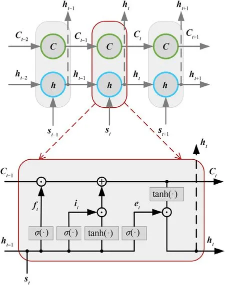
Fig.4.Structure of LSTM networks.

An LSTM network, unlike traditional recurrent networks, contains a new internal state C and three gates: forgetting gate,input gate i,and output gate e.The following equations can calculate Ctand htat a specific time.

where

W（·）and b（·）are the trainable parameters of an LSTM network.

3.Guidance law implementation

The proposed RRTD3 algorithm is first introduced in this section, followed by implementation details based on the aforementioned engagement scenario.

3.1.Recorded recurrent twin delayed deep deterministic policy gradient

3.1.1.Whatisdeterministicpolicygradient?

In RL, the ultimate goal of an agent is to optimize its policy by maximizing the episode reward shown in Eq.(3).The state-value function and action-value function can be defined for a specific policy as follows:

The state-value function vπ（xt） represents the expected reward of implementing policy π starting from state xt, and the actionvalue functionqπ（xt，ut） denotes the expected reward of adopting policy π after taking action uton state xt.Obviously,bothqπ（xt，ut）and vπ（xt）can be used to evaluate policy π.An optimal policy π*can be easily obtained given an optimal state-value function v*（xt）or an optimal action-value functionq*（xt， ut）.Takingq*（xt，ut） as an example, we have

In general, it is challenging to obtain v*（xt） andq*（xt，ut） directly,and parameterized models are usually used to approximate them.For example, a functionqπ（xt，ut;w） orqπ（ot，ut;w） in a POMDP,with parameter w, can be used to approximate the action-value function.In training, policy evaluation and improvement are repeated to improveqπ（ot，ut;w） continuously and, as a result,optimize policy π.Many value-based RL algorithms,such as deep Qnetwork (DQN)[35], are based on the above idea.

However, value-based algorithms are best suited to discrete problems with a limited number of actions.For continuous problems, policy-based algorithms are a better choice.A policy-based algorithm also uses parameterization to train a policy π（ut|ot;θ）with parameter θ.In training, the parameter is updated with the aim of maximizing a certain objective functionJπ（θ） , so θ may be updated by gradient ascent as follows:

where αθis the learning rate of θ, andJπ（θ） can be defined as

The policy gradient ∇θJπ（θ） may be calculated using the policy gradient theorem as follows:

In order to apply the policy gradient theorem,it is common practice to estimateqπθ（xt，ut） in Eq.(18) via a Monte Carlo method.However, this estimate is only updated after the end of an episode.To this end, a parameterized value functionqπθ（ot，ut;w） can be used to approximateqπθ（xt，ut）so that the update does not have to wait until the end of an episode, which is the basic idea of actor-critic algorithms.

Strictly speaking, the policies mentioned above map observations to the selection probabilities of actions.For a continuous space,the number of actions is infinite,so it is not feasible to get the selection probability of each action.To this end, the deterministic policy,which means ut=π（ot;θ）,was proposed.Based on Eq.(18),the gradient of a deterministic policy is derived as

and for actor-critic algorithms, Eq.(19) is further rewritten as

3.1.2.Whatistwindelayeddeepdeterministicpolicygradient?

The so-called DRL means that both the parameterized policy π（ot;θ）and the action-value functionqπθ（ot，ut;w）are respectively implemented by a deep neural network,i.e.,policy network and Qnetwork.The twin delayed deep deterministic (TD3) policy gradient is derived from the aforementioned deterministic actorcritic algorithm using the dual DQN idea.Due to the poor training stability of classical actor-critic algorithms, TD3 adopts the experience-replay and target-network mechanisms in DQN.

The experience-replay mechanism means that the experience data （ot，ut，rt，ot+1） obtained from each interaction between the agent and the environment is collected and stored in an experience pool D.When there is enough data in D,a small batch of data B =｛（oj，uj，rj，oj+1）1，...，（ok，uk，rk，ok+1）B｝ is randomly sampled to update the network parameters, whereBis the length of data set B.The target-network mechanism means that in addition to the conventional policy network π（ot;θ） and Q-networkqπθ（ot，ut;w）,we introduce their respective target networks, namely, the target policy network π（ot;θtar）and the target Q-networkqπθ（ot，ut;wtar）.Both these two mechanisms can effectively improve algorithm training stability and thus accelerate convergence.Nevertheless,the problem of overestimating the value function persists.To this end,TD3 employs the idea of twin Q-networks in dual DQN.During training,the two Q-networks,are updated concurrently, and the smaller of the two is chosen as the value function estimate.In this way,a total of six networks are used in TD3: the policy network π（ot;θ）, the target policy network π（ot;θtar）, the Q-networksand the target Q-networks.

In DRL, updating the policy network parameter aims at maximizing the reward,so the following loss function is defined for the policy network.

The loss functions of the Q-networks are similar to DQN and are defined as follows:

Moreover,ycan be calculated by

where ε ～clip（N（0，σ2），-c，c）is artificial noise used to increase the robustness of the value function estimation.

The network parameters θ and wican be updated based on the above loss functions via Eq.(24).

αθand αware the learning rates of θ and wi, respectively.The target networks are softly updated according to Eq.(25)to prevent them from changing too much.

and αtaris the soft-update factor.

Updates to the policy and target networks are delayed to increase training stability.Concretely,they are only updated once perpupdates to the Q-networks.In addition, given that the policy in TD3 is deterministic, it is necessary to append noise to the action determined by the policy π（ot;θ） to ensure that the agent is sufficiently exploratory,i.e.,ut=π（ot;θ）+N ,where N ～-ns，ns）.

3.1.3.Whatisrecordedrecurrent?

For a defender,measurement noise or an infrared seeker results in a partially observable training environment,known as a POMDP,which degrades the performance of classical TD3 significantly.On the other hand, the detection frequency of a defender is usually higher than its guidance frequency, i.e.,multiple measurements at different moments are available within each guidance cycle.Inspired by the above observations,we insert an RNN layer into the policy network and feed the sequence measurements within each guidance cycle into this recurrent layer to extract additional temporal information about the input.In this paper, an LSTM network is chosen as the recurrent layer.

Using an RNN layer in the policy network enables the agent to fully utilize the measurement data and mitigate the negative impact of the training environment’s partial observability.Furthermore, it also helps to improve the policy’s generalization,i.e.,its adaptability to different scenarios.Nevertheless,it brings a new problem,namely the partial observability of the agent itself.After feeding the sequence observation otto the RNN layer in the policy network,the RNN layer mines the temporal information of otthrough its internal hidden state htand transmits htto the following layers of the policy network.In other words, the input of the policy network now comprises not just the observation otbut also the temporal information of otembedded in the hidden state ht.However,the input of a conventional Q-network in TD3 only contains the observation otand action ut,but not the temporal information of ot,which results in partial observability of the agent itself.

To this end,the RRTD3 algorithm is proposed in this paper.After each interaction with the environment in training,the hidden state htof the RNN layer in the policy network is recorded and utilized as a part of the new Q-networksinput.The target Qnetworks are changed toaccordingly.Spontaneously, the format of the experience data stored in D changes to（ot，ut，ht，rt，ot+1） instead of （ot，ut，rt，ot+1）.The proposed RRTD3 preserves the benefits of employing an RNN layer in the policy network while overcoming partial observability inside the agent,resulting in improved training stability.

In summary, we have the following algorithm:

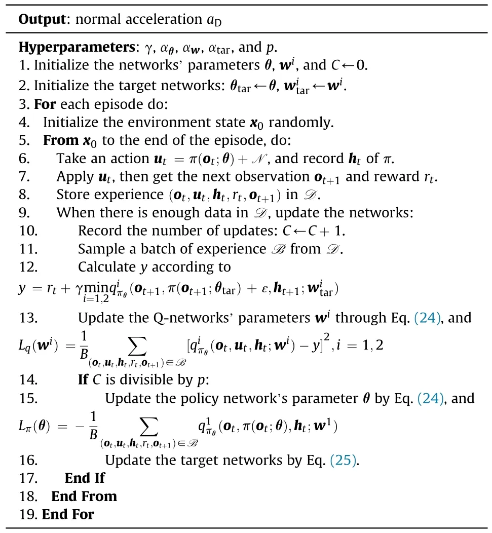
Algorithm 1. RRTD3-based interception guidance law.

3.2.Implementation details

Fig.5 depicts the data flow diagram in training,which combines the proposed RRTD3 algorithm with the engagement scenario described in subsection 2.2.As illustrated in Fig.5, the training environment comprises observation uncertainty in addition to random initialization, random heading error, and maneuverability uncertainty, which can help the policy network cope better with measurement noise in an actual engagement.Let ogbe the observation obtained from the engagement geometry at a particular moment, and then we can get the noisy observation by

Furthermore, for RRTD3, the reward functionrtin Fig.5 is critical, affecting its convergence speed and even feasibility.In this paper,reward shaping is introduced to designrt,and the designed reward function is

and

Fig.5.Data flow diagram in training.

where β（·）and σ（·）are hyperparameters,ΔqDM=qDM-.

In Eq.(27),rshapingis the designed shaping reward.Given that the defender flies slower than the missile, the classical parallel approach method is employed in designingrshaping.To raisershaping,the agent must decrease |ΔqDM| and |ΔqDM|, i.e., strive to keep the defender-missile LOS angle constant.It is consistent with the parallel approach method.The last term ofrshapingencourages the defender to minimize energy consumption.renddenotes the reward at the end of an episode.IfrDM≤Rmiss, i.e., the defender successfully intercepts the missile,and the agent receives a positive reward β4; conversely, the agent cannot get any reward for a failed interception.

In this paper,we investigate the following five different cases to verify the proposed RRTD3's performance.

Case 1: The observation only contains angular information at a single moment.

Case 2:The observation contains range and closing velocity at a single moment in addition to angular information.

Case 3: The observation contains sequential angular information, i.e., measurements over multiple moments.

Case 4: The observation is sequential and contains information on the angle, range,and closing velocity.

Case 5: The hidden state of the policy network is not recorded,i.e., the input of the Q-network does not contain ht.

Case 1 and Case 2 can be trained using the classical TD3 algorithm due to their non-sequential observations,implying that their policy networks do not comprise LSTM layers.Case 3 and Case 4 are trained through the proposed RRTD3 algorithm, and Case 5 is utilized to evaluate the effect of recording htduring training.The policy networks and Q-networks for these five cases are designed as follows.

3.2.1.Policynetworks

A policy network maps an agent's observation directly to its action.The defender in Case 1 is assumed to be using an infrared seeker that solely measures angular information, so the observation in Case 1 is designed as

The defender in Case 2 is assumed to adopt a radar seeker capable of measuring range, closing velocity, and angular information.Therefore,the observation in Case 2 is

The observations in Case 3 and Case 5 are the same, i.e., the sequential angular information shown in Eq.(32).

The policy networks’ inputsare generated through processing each of the observations above according to Eq.(26),wherek=1，...，5.It is worth noting that the outputs of the policy networks in all five cases above are the normal acceleration of the defender,i.e.,

The architecture of policy networks for these five cases may be constructed as indicated in Table 2 based on the above-defined observations and actions.Since the observations of Case 1 and Case 2 are non-sequential, their policy networks are both composed of a fully connected network with three hidden layers but no LSTM layer.The observations of Case 3,Case 4,and Case 5 are sequential, so their policy networks each include one LSTM layer followed by three fully connected layers.In addition,given that the actions shown in Eq.(34)are bounded,the output layers'activation functions of all policy networks are set to tanh to restrict the outputs.The hidden layers’activation functions are all ReLU,which is defined as

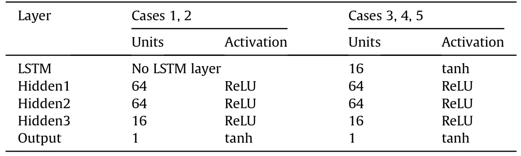
Table 2Architecture of policy networks.

3.2.2.Q-networks

The construction of the Q-networks in Case 1 and Case 2 is simple.In Case 1, the Q-network's input is, while in Case 2,it is.They are both one-dimensional vectors.So the Q-networks of Case 1 and Case 2 can be designed as simple fully-connected networks shown in Table 3.

However, the problem becomes more complicated in the other three cases because the Q-networks’ inputs comprise onedimensionalut, ht, and two-dimensional ot.To this end, we design the architecture illustrated in Fig.6 for the Q-networks of these three cases, where Input1 is two-dimensional and Input 2 is one-dimensional.Input 1 in Case 3, Case 4, and Case5 are,respectively.Input 2 in Case 3 and Case 4 is［ut，ht］T∈R17,but it isut∈R in Case 5 and does not contain the hidden state of the policy network.In addition, the activation functions of all hidden layers in Fig.6 are ReLU.On the other hand,the activation functions of the LSTM layer and output layer are tanh and linear, respectively.

4.Numerical simulation

In this section, training is conducted in each of the five cases above, and numerical tests for the policies generated from the training are carried out in various scenarios to test the proposed RRTD3 adequately.

4.1.Training process

A fourth-order Runge-Kutta integrator is utilized to update the training environment with an integration step of 0.01 s ifrDM＞500 m and 0.0001 s otherwise.The defender and the missile have 20 Hz guidance frequencies, whereas the defender’s seeker has a detection frequency of 100 Hz, resulting inM=5 in Eqs.(32) and(33).Let the experience pool D capacity be |D| = 500000, and the networks are only updated when the amount of data stored in D exceeds|D|/10.Furthermore,during the first 5000 episodes,the boundnsof action noise N gradually decreases from 0.05 to 0 to balance exploration and utilization throughout training.Table 4 lists all hyperparameters used in training.

The initial states of both the defender and the missile arerandomly initialized in training, as indicated in subsection 2.2, to ensure the generalization of the resulting policies.The defender also suffers from maneuverability uncertainty and observation noise,as shown in Eqs.(10)and(26),respectively.In addition,as a baseline in training, we introduce a new case that contains the same elements as Case 2 but does not include maneuverability uncertainty and observation noise.The training curves of the baseline and the other five cases are shown in Fig.7.Fig.7(a) depicts the trend of the average reward obtained by the agent for each interaction with the environment in one episode.At the same time,Fig.7(b) gives the interception rate of the policy obtained after a different number of episodes of training under 500 Monte Carlo simulations.

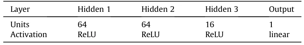
Table 3Architecture of Q-networks for cases 1 and 2.

As shown in Fig.7(a),the average reward for Case 1 and Case 2 not only lifts later relative to the baseline but also converges to a significantly smaller stable value.It is mainly due to the observation noise that makes the environment partially observable and the uncertainty of the defender's maneuverability.Compared to Case 1 and Case 2, the average rewards of Case 3 and Case 4 are boosted earlier and can converge to larger values.It means that utilizing LSTM layers increases data efficiency and speeds up training while simultaneously mitigating the adverse effects of partial observability on DRL, allowing agents to gain greater rewards and hence better policies.It also can be seen that the training curves of Case 3 and Case 4 are similar,implying that even if the defender can only obtain angular information, it will have an interception rate comparable to that of using a radar seeker.It is attributed to both the proposed RRTD3 and the shaping reward.In Case 5, the agent's performance fluctuates significantly, even though it can occasionally acquire big rewards.Fig.7(b)further indicates that the training in Case 3 and Case 4 is significantly more stable than in Case 5,thanks to the proposed approach of recording the hidden state htduring training.

In summary, the proposed RRTD3 algorithm 1) improves data utilization, and training speed, 2) mitigates the adverse effects of partial observability, 3) enhances training stability: (a) Average reward; (b) Interception rate.

4.2.Numerical tests

In order to verify the performance of the designed RRTD3-based interception guidance laws, the following numerical tests are conducted on the policy networks obtained from the above training process.

4.2.1.Testsinthetrainingscenario

The tests are first conducted in the same setting as the training environment presented in subsection 2.2,with the PNG and APNG from Eq.(36) as a comparison.

wherekPN=6.0,kAPN=3.0,anddenotes an estimation of the missile’s acceleration.

Table 5 and Fig.8 are the testing results in the training scenario.The policy networks acquired in Case 1 and Case 2 are denoted by TD31and TD32,respectively.RRTD31and RRTD32correspond to the policy networks obtained in Case 3 and Case 4,respectively.Given that the agents in Case 1 and Case 3 cannot acquire,while the agents in Case 2 and Case 4 can, it is apparent that it is more reasonable to compare PNG with TD31and RRTD31and APNG with TD32and RRTD32,respectively,for the sake of fairness.It is exactly whyVDis used in PNG instead of.

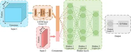
Fig.6.Architecture of the Q-network with an LSTM layer.

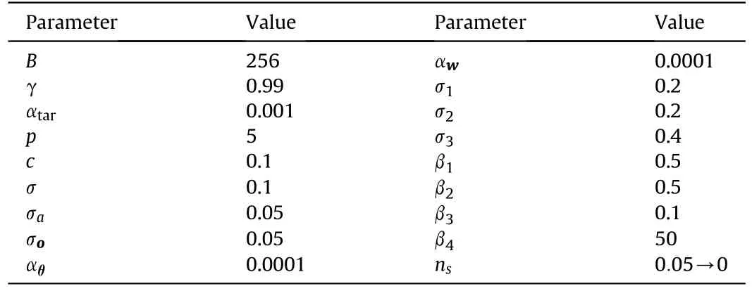
Table 4Hyperparameters.

Fig.7.Training curves.

A typical engagement scenario is illustrated in Fig.8,where the initial defender-missile distance= 16728 m, the LOS angle= 88.10°, and the defender’s heading errorHE= 10°.As shown in Fig.8(a),both RRTD31and RRTD32successfully intercept the incoming missile with a miss distance of 0.299 m and 0.077 m,while PNG and APNG fail to intercept with a miss distance of 25.915 m and 20.334 m, respectively.Combining the command information given in Figs.8(b) and 8(c), it can be seen that at the beginning of the engagement, the main effort of the defender is devoted to correcting the heading error.WhenrDMis small enough,and the missile starts to execute an evasive maneuver,both RRTD31and RRTD32react to this maneuver sufficiently to intercept successfully.Contrastingly,the PNG does not react at all to the missile’s evasive maneuver,while the APNG does react somewhat,but this is very limited and insufficient to intercept.Monte Carlo tests are conducted to further explore the performance of different guidance laws.

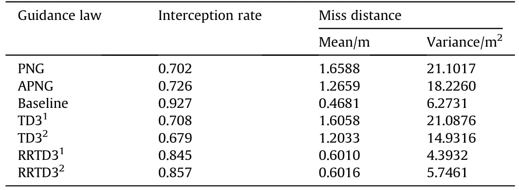
Table 5Statistical comparison of different guidance laws.

Table 5 shows the statistical comparison of the different guiding laws after 1000 Monte Carlo tests.Baseline’s test results show that the classical TD3 algorithm can be trusted to train a highperforming policy network with an interception rate of over 90%without considering uncertainties and partial observability of the training environment.However, the test results of TD31and TD32reveal that the performance of the policy networks trained by the classical TD3 algorithm drops significantly to the same level as the PNG once the uncertainties or partial observability are present.

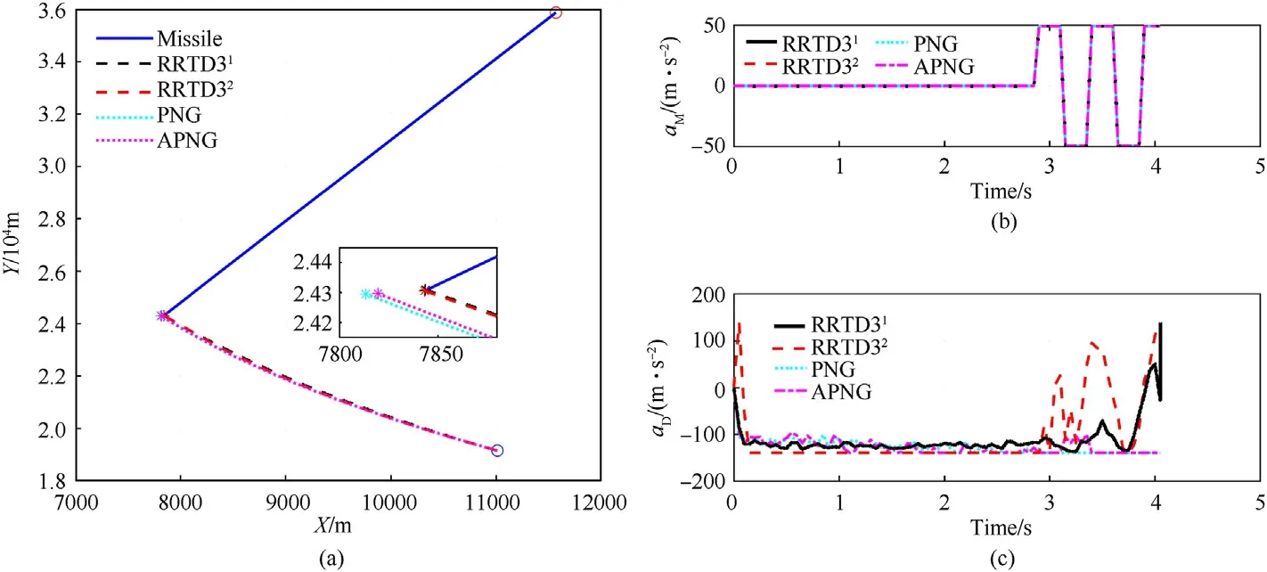
Fig.8.A typical engagement scenario: (a) Trajectories; (b) Missile acceleration; (c) Defender acceleration.

As shown in Table 5, the interception rates of TD31and TD32decrease by more than 20% compared to Baseline.Meanwhile, the means and the variances of miss distances increase by more than 150% and 130%, respectively.The above results corroborate the bottleneck of the classical TD3 algorithm when facing a partially observable environment with uncertainties.Conversely, training through the proposed RRTD3 can significantly improve the performance of the resulting policies and overcome the aforementioned bottleneck of the classical TD3 algorithm.The test results indicate that compared to TD31and TD32,the interception rates of the RRTD3-based policies RRTD31and RRTD32are both improved by around 20%.At the same time, the means and the variances of miss distances are reduced by up to 62.6% and 79.2%, respectively.Given that many interceptors intercept missiles through the hit-tokill technique, it is evident that a smaller miss distance is more conducive to achieving it.In addition, more minor miss distance variances indicate that the RRTD3-based guidance laws perform smoothly without excessive fluctuations in the face of different engagement geometries.The above analysis verifies the advantages of the proposed RRTD3 over classical TD3 in coping with uncertainties and partial observability,which is consistent with what is reflected in Fig.7.

4.2.2.Generalizationtounseenscenarios

The above tests demonstrate the advantages of the policies trained by RRTD3 in the training scenario, while tests on the policies’ adaptability to some novel unseen scenarios, i.e., generalizability, are carried out in this part.The tests are divided into two aspects.The first aspect tests the performance of the RRTD3-based guidance laws for different initial heading errors.Varying,the performance of different guidance laws is obtained,as illustrated in Figs.9 and 10.The interception rates are shown in Figs.9,and Fig.10 shows the statistical characteristics of miss distances.The second aspect is used to evaluate the guidance laws’interception rates for missiles with different maneuver modes, which is achieved by changing the missile’s maneuver frequency.The normal displacementaMΔt2/2 of the missile increases when its maneuver frequency decreases,implying that the missile has a larger maneuver area.The corresponding interception rates at different maneuver frequencies are shown in Fig.11.

Fig.9.Interception rates with different initial heading errors.

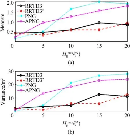
Fig.10.Miss distances with different initial heading errors: (a) Mean; (b) Variance.

According to Figs.9 and 10, it can be seen that unless it is an ideal no-heading-error scenario, the RRTD3-based guidance laws consistently possess higher interception rates and smaller miss distances relative to PNG and APNG for different initial heading errors.Furthermore, the testing results further illustrate that the RRTD3-based guidance laws have more pronounced advantages asincreases, i.e., they can cope with more significant initial heading errors.It means that the proposed guidance laws reduce the requirement for the defender’s midcourse guidance accuracy,thereby reducing the design difficulty of the midcourse guidance law.

Fig.11.Interception rates with different evasive maneuver frequencies: (a) ωM =360°/s; (b) ωM = 180°/s; (c) ωM = 90°/s.

Thus far, the tests seem to indicate that there is no significant difference in performance between RRTD31, which relies only on angular information, and RRTD32, which relies on both angular information, range, and closing velocity.Obviously, it defies our common sense,and Fig.11 reveals the difference between them.As seen in Fig.11, even if the missile’s evasive maneuver mode changes, RRTD32has an interception rate comparable to that of APNG.Moreover, the performance of RRTD32does not decay excessively as the maneuver frequency decreases.It indicates that RRTD32can overcome initial heading errors and effectively intercept missiles maneuvering over large areas.Given the optimality of APNG against maneuvering targets [51], the fact that RRTD32can have the same excellent performance as APNG without additional acceleration information fully demonstrates the advancement of the proposed algorithm.However, the test results of RRTD31in Fig.11 contradict the above findings.As the missile maneuver area expands, the interception rate of RRTD31decreases significantly,even worse than PNG,which is significantly different from RRTD32.The fundamental reason for this discrepancy is undoubtedly the difference in observation.The maneuver mode shown in Eq.(9)implies that the missile executes a significant maneuver to evade the defender only when it is very close to the defender.This evasive maneuver will inevitably cause a sharp change inqDMandresulting in a drastic change in the output of RRTD31, whose observation contains angular information only, thus reducing its interception rate.Contrastingly, while the observation of RRTD32containsqDMand, it also containsrDMandandchange less severely when the missile performs a significant maneuver,so their presence in the observation can somewhat mitigate the adverse effects of the drastic changes inqDMand, thus ensuring the interception rate of RRTD32does not significantly degrade.Further,the above analysis fits our common sense,i.e.,the adequate information available, the better.

It should be added that the policy networks RRTD31and RRTD32obtained based on the proposed RRTD3 algorithm both consist of one LSTM layer and three fully connected hidden layers,containing 7521 and 7669 parameters,respectively.Moreover,the dimensions of the observations areand, respectively.In practice, only up to 7669 double data need to be stored using the above policy networks, which usually occupy only about 61 KB of memory.In addition, the computer only needs to perform simple nonlinear and matrix multiplication operations to map the observations to actions,which has been tested to be less than 0.05 ms on a 3.80 GHz CPU by C++.The above shows that the proposed RRTD3-based guidance laws are computationally less burdensome and have the potential to run on modern flight computers.

4.3.An extended scenario

The test results in Fig.11 preliminarily reveal the effect of observation on the agent’s behavior.An extended scenario is investigated in this subsection to analyze further the criticality of observation and reward on the agent’s behavior in DRL.In this scenario,the shaping reward is no longer in the form shown in Eq.(28)but becomes Eq.(37)related to the remaining flight time.The difference between the two is that the former encourages the defender to intercept the missile in a near-parallel approach, while the latter induces a minimum-time interception.

Wheretgo= -, σ4=4.0 is a hyperparameter.For comparison, two cases with different observations are investigated in this scenario:Case 6 and Case 7.Their observations are the same as those of Case 3 and Case 4, i.e.,

It means that the observation of Case 6 contains only angular information, while the observation of Case 7 has additional range and closing velocity.

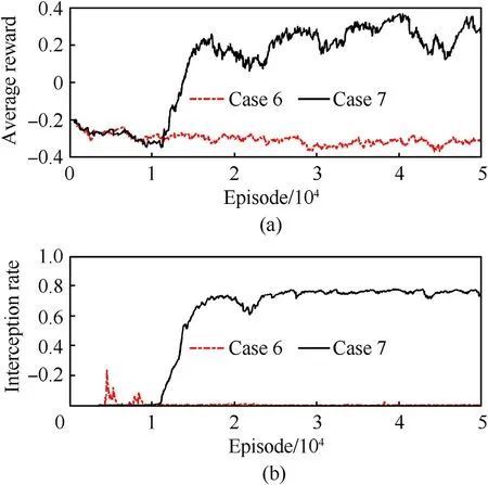
Fig.12.Training curves of the extended scenario:(a)Average reward;(b)Interception rate.

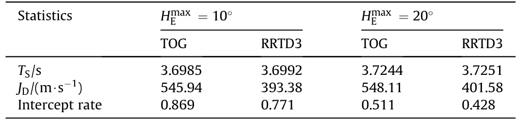
Table 6RRTD3-based guidance law versus TOG.

The other hyperparameters are the same as those in subsection 4.1.After 50,000 episodes, the training curves of this extended scenario are shown in Fig.12, where the subplots have the same meaning as those in Fig.7.In this scenario,the average reward and interception rate of Case 7 gradually increase after 11,000 training episodes and converge after 25,000 episodes.Contrastingly, the training curves of Case 6 remain low and do not rise significantly with the training runs.The explanation for this can be found in the perspective of matching rewards and observations.Considering the training curves Figs.7 and 12 together, as well as the shaping reward Eqs.(28) and (37).It can be seen that Eq.(28) relies on angular information.In contrast, Eq.(37) relies on the range and closing velocity.Therefore,in the scenario with the shaping reward Eq.(28),even Case 3,where the observation contains only angular information, can obtain a policy network with excellent performance after sufficient training.However, in the extended scenario with the shaping reward Eq.(37), the observation containing only angular information cannot match the reward shown in Eq.(37),which is the reason why the performance of the agent in Case 6 cannot be improved.The above analysis reveals the importance of observation-reward matching in DRL, where unreasonable observations and rewards may cause non-convergence.

Since the shaping reward Eq.(37) induces a minimum-time interception, in the following, we may wish to compare the guidance law obtained by Case 7 with a traditional time-optimal guidance (TOG) law [52] to verify the suboptimality of DRL [53].To more comprehensively illuminate the performance differences,we define the following index.

5.Conclusions

This paper proposes a novel deep reinforcement learning algorithm called RRTD3 for developing guidance laws for intercepting endoatmospheric maneuvering missiles.A typical engagement scenario containing a target, missile, and defender is first presented,followed by the establishment of a training environment for reinforcement learning based on the derived kinematic equations of this scenario.Given the fact that the speed of the defender is lower than that of the missile,a reward function is designed based on the classical parallel approach method.Random initialization,observation noise,and maneuverability uncertainty are introduced in the training environment to guarantee the generalization of the resulting policies, which in turn makes the environment partially observable,so the RRTD3 algorithm is proposed.It is implemented by inserting an LSTM layer at the end of the policy network near the input.All measurements acquired at different detection moments within a guidance cycle are unified into a sequence observation and fed into the policy network.Taking advantage of the LSTM networks in processing sequential data to exploit the temporal information implicitly inside the observation mitigates the negative impact of partial observability while simultaneously improving data utilization and speeding up the training.Nevertheless, the partial observability inside the agent caused by introducing the LSTM layer cannot be ignored.Therefore, recording the hidden states of the LSTM layer in the policy network during training is proposed, which eliminates the partial observability problem inside the agent completely and thus makes the training process smoother.

The simulation experiments consider two different types of defenders employing an infrared or radar seeker.Comparing the training curves of five different cases and one baseline, the advantages of the proposed RRTD3 in terms of training efficiency,training stability, and performance of the resulting policy are verified.The test results illustrate that compared to some classical guidance laws, RRTD3-based guidance laws have higher interception rates,smaller miss distances,and more stable performance in different scenarios,regardless of which seeker is used.In addition,they can reduce the requirement for midcourse guidance accuracy with a small computational burden.Meanwhile, simulations in an extended scenario validate the suboptimality of DRL and reveal the importance of observation-reward matching for DRL.In future studies, it may be feasible to use explainable reinforcement learning to address the open topic of designing reasonable observations and rewards in DRL.

Declaration of competing interest

The authors declare that they have no known competing financial interests or personal relationships that could have appeared to influence the work reported in this paper.

Acknowledgments

This work was supported by the National Natural Science Foundation of China (Grant No.12072090).