Roles of Equatorial Ocean Currents in Sustaining the Indian Ocean Dipole Peak

XING Huibin, WANG Weiqiang, WANG Dongxiao, and XU Kang

Roles of Equatorial Ocean Currents in Sustaining the Indian Ocean Dipole Peak

XING Huibin1), 2), WANG Weiqiang1), 3), 4), *, WANG Dongxiao5), and XU Kang1), 3)

1) State Key Laboratory of Tropical Oceanography, South China Sea Institute of Oceanology, Chinese Academy of Sciences, Guangzhou510301, China 2) University of Chinese Academy of Sciences, Beijing100049, China 3) Southern Marine Science and Engineering Guangdong Laboratory (Guangzhou), Guangzhou511458, China 4) Innovation Academy of South China Sea Ecology and Environmental Engineering, Chinese Academy of Sciences, Guangzhou511458, China 5) School of Marine Sciences, Sun Yat-sen University, Zhuhai 519082, China

In this study, on the basis of the results of the European Centre for Medium-Range Weather Forecasts Ocean Reanalysis System 4, the response of equatorial ocean currents and their roles during the peak phase of the Indian Ocean Dipole (IOD) are comprehensively explored. During the IOD peak season, a series of ocean responses emerge. First, significant meridional divergence in the surface layer and convergence in the subsurface layer are found in the equatorial region. The equatorial easterly winds and off-equatorial wind curl anomalies are found to be responsible for the divergence at 55˚–80˚E and the convergence at 70˚–90˚E. Second, the meridional divergence and convergence are found to favor a weakened Wyrtki jet (WJ) in the surface layer and an enhanced Equatorial Undercurrent (EUC) in the subsurface layer, respectively. Therefore, these ocean responses provide ocean positive feedback that sustains the IOD peak as the weakened WJ and enhanced EUC help maintain the zonal temperature gradient. Additionally, heat budget analyses indicate that the weakened WJ favors sea surface temperature anomaly warming in the western Indian Ocean, whereas the enhanced EUC maintains the sea surface temperature anomaly cooling in the eastern Indian Ocean.

surface divergence; subsurface convergence; equatorial zonal currents; the Indian Ocean Dipole; positive feedback

1 Introduction

The Indian Ocean Dipole (IOD) is a major interannual mode associated with the significant oscillation of the local ocean-atmosphere state over the tropical Indian Ocean (TIO; Saji, 1999; Vinayachandran, 1999; Webster, 1999; Saji, 2018). A positive IOD is characterized by a negative sea surface temperature anomaly (SS- TA) in the southeastern Indian Ocean and a positive SSTA in the western Indian Ocean. The IOD usually develops from June and reaches its peak in boreal fall. During the IOD peak, strong easterly wind anomalies appear along and south of the equator with accompanying anomalous southeasterly along-shore winds off the Sumatra-Javacoast. In addition, a pair of anticyclonic wind stress anomalies exist in the off-equatorial region (Rao and Behera, 2005; Yu, 2005).

The evolution of the IOD has four main feedback mech-anisms. First, the Bjerknes feedback proposed by Bjerknes (1969) to explain the development of an El Niño-South- ern Oscillation (ENSO) event has been applied to IOD development (Yamagata, 2004). During a positive IOD event, a west-east dipole SSTA pattern exists in the TIO. Anomalous easterly winds prevail along the equator when the sea surface temperature (SST) is cool in the east and warm in the west. The thermocline depth shoals in the east and deepens in the west in response to easterly winds. These oceanic and atmospheric conditions imply that a Bjerknes feedback-type mechanism is responsible for the IOD evolution. Second, ocean waves also play important roles in IOD development. The equatorial Kelvin waves induced by the anomalous easterly winds and the off-equa- torial Rossby waves induced by anomalous anticyclonic wind stress are potentially important for the establishment of the zonal temperature gradient during IOD events (Huang and Kinter III, 2002; Rao, 2002; Xie, 2002; Feng and Meyers, 2003; Delman, 2016). The third and fourth mechanisms are the wind-evaporation-SST (WES) feedback (Xie and Philander, 1994) and SST-cloud-radiation (SCR) feedback, both of which can influence the IOD in the developing and decaying periods. During the developing period, the ocean loses much latent heat with an increase in wind speed and the cool SST in the eastern basin (Li, 2003). During the decaying period, the anomalous winds are against the climate state, and the wind speed decreases. The ocean loses minimal latent heat because of the decrease in wind speed. Such loss contributes to the increase of the SST in the eastern basin. Furthermore, the negative SSTA weakens the local convention, and the cloud cover is much less than that in the normal state. A large amount of solar shortwave radiationreaches the ocean and dampens the negative SSTA growth.

Equatorial zonal currents in the TIO are enigmatic and are mainly characterized by transient currents that maintain the basin-scale water mass and heat balance. The equatorial currents, including the Wyrtki jet (WJ; Wyrtki, 1973) and Equatorial Undercurrent (EUC; Knauss and Taft, 1964) occur twice a year during the monsoon transition periods. The WJ and EUC are important oceanic features in the equatorial region, and they are particularly important in the TIO because of their transient nature. In addition, the WJ and EUC show strong quasi-biannual variability, which is most pertinent to the occurrence of IOD events (Nagura and McPhaden, 2008; Nyadjro and McPhaden, 2014; Nagura and McPhaden, 2016; Sachidanandan, 2017; Gnanaseelan and Deshpande, 2018). The weakened WJ in response to surface winds reduces eastward water and heat exchange, which is responsible for IOD development (Chowdary and Gnanaseelan, 2007; Nagura and McPhaden, 2010; Gnanaseelan, 2012; McPhaden, 2015). The EUC normally exists in the western Indian Ocean, but it can extend to the eastern basin during positive IOD events (Reppin, 1999; Iskandar, 2009; Zhang, 2014; Chen, 2015; Rao, 2017a). The enhanced EUC significantly reinforces the IOD through coastal upwelling in the eastern basin (Chen, 2016a).

Compared with the WJ and EUC, equatorial meridional currents are much weaker and have stronger intraseasonal variability; moreover, their interannual variability has re- ceived less attention (Rao, 2017b). Recent studies have revealed poleward transport anomalies in the mixed layer and equatorward anomalies in the subsurface layer in the equatorial region during the IOD peak (Krishnan and Swapna, 2009; Sun, 2014; Zhang, 2014). Nonetheless, the basic features of equatorial meridional currents, especially their roles in the IOD, are not clear and have yet to be systematically investigated.

To study the importance of equatorial ocean currents in sustaining the zonal temperature gradient during the IOD peak, comprehensive details of their basic characteristics and the dynamic linkages between equatorial zonal and meridional currents need to be obtained. Moreover, the oceanic processes during the IOD peak should be systematically explained.

The aim of the current study is to examine the responses of equatorial ocean currents and their roles in sustaining the zonal temperature gradient during the IOD peak in the TIO. The remainder of the paper is organized as follows. Section 2 describes the data and methods used in this study. Section 3 presents the results. Section 4 provides a summary and discussion.

2 Data and Methods

2.1 Ocean Reanalysis Data

In this work, monthly outputs from the European Centre for Medium-Range Weather Forecasts (ECMWF) Ocean Reanalysis System 4 (ORAS4) from January 1958 to December 2017 are used to analyze the responses of equatorial ocean currents and their positive feedback during the IOD peak. The details of the ORAS4 are fully described in the work of Balmaseda(2013); herein, we only list key information. The ORAS4 utilizes the third version of the Nucleus for European Modeling of the Ocean model, and the assimilation window is ten days (Madec, 2008). The assimilated observations include the data from expendable bathythermographs, conductivity-temperature-depth sensors, mooring buoys, autonomous pinniped bathythermograph, altimetry, and Argo floats. No assimilation is used for the velocity observations.

The ORAS4 is forced by daily surface fluxes, momentum, and freshwater flux. Wind stresses and surface flux forcings are obtained from the ECMWF Re-Analysis 40 (ERA40, Uppala, 2005) before 1989, the ERA-Interim Reanalysis (Dee, 2011) from January 1989 to December 2009, and the operational ECMWF atmosphericanalysis from January 2010 onwards. The heat flux is corrected by a strong relaxation to gridded SST productsa relaxation coefficient of 200Wm–2℃–1. In addition, the evaporation minus precipitation is adjusted globally by constraining the global-model sea-level changes to the changes derived from altimeter data and locally by relaxation to monthly climatology of surface salinity from the WOA05. The horizontal resolution of the ORAS4 is 1.0˚×1.0˚ and the model has 42 nonuniform vertical levels(18 levels in the upper 200m). The ORAS4 has been found to be the best reanalysis product over the Indian Ocean among all available products (Karmakar, 2017).

The wind data used to analyze the causes of meridional divergence and convergence are from the joint winds from the ERA40 (January 1958 to December 1989) and ERA-Interim (January 1990 to December 2017). The surface heat fluxes for heat budget analysis are also from the ERA40 and ERA-Interim, which has been assessed as a suitable observed product to choose (Zhang, 2018).

Three sets of data are used to check the interannual variabilities of the meridional currents and their relationship with the equatorial zonal currents. The Estimating the Circulation and Climate of the Ocean Phase II (ECCO2) developed by the Jet Propulsion Laboratory for the period of 1992–2012 has a 0.25˚ horizontal grid. The Simple Ocean Data Assimilation version 3.4.2 (SODA3.4.2) is built on the Modular Ocean Model v5 ocean component of the Geophysical Fluid Dynamics Laboratory CM2.5 coupled model (Carton, 2018). SODA3.4.2 does not assimilate velocity information and thus provides the opportunity to conduct an independent check of the ocean reanalysis velocity. SODA3.4.2 has a 0.5˚ horizontal grid and spans the period of 1980–2016. The Community Earth System Model version 1 (CESM; Hurrell, 2013) in-cludes coupled atmosphere, ocean, land, and sea ice components, all with a horizontal resolution of about 1˚. The oceanic component, the Parallel Ocean Program version 2 (POP2; Smith, 2010), has 60 vertical layers. In this study, a fully coupled model is run using preindustrial conditions. The model runs 1200 years to reach a stable state. The last 200 years are used for comparison.

In addition, the dipole mode index (DMI) used here is derived from the difference in the SSTAs of the tropical western Indian Ocean (50˚–70˚E, 10˚S–10˚N) and southeastern Indian Ocean (90˚–110˚E, 10˚S–0˚) following the work of Saji(1999). On the basis of the DMI, 12 positive IOD events are chosen using a threshold of 0.5℃for the following composite analysis. These IOD events are 1961, 1963, 1967, 1972, 1977, 1982, 1994, 1997, 2006, 2011, 2012, and 2015.

2.2 Methods

All variables used are detrended to remove low-frequency signals. Then, the monthly climatology is subtracted so as to obtain the monthly anomalies. The data are further smoothed with a three-month running mean to remove the intraseasonal signals.

First, we examine the responses of the anomalous meridional currents during the IOD peak. The main features are meridional divergence in the surface layer and convergence in the subsurface layer (Fig.1a). Hence, the surface layer is defined as the mixed layer, and the subsurface layer is defined as the layer between the base of the surface layer and the depth of the 20℃ isotherm (D20). The mixed layer depth (MLD) is defined as the depth at which the potential density increases from the surface value because of a temperature decrease of Δ=0.5℃ (de Boyer Montégut, 2004).

Heat budget was calculated for Box A (50˚–70˚E, 10˚S–10˚N) and Box B (90˚–110˚E, 10˚S–0˚) in the surface layer and for Box C (90˚–110˚E, 10˚S–0˚) in the subsurface layer to verify the relative contributions of ocean processes in sustaining the zonal temperature gradient during the IOD peak. On the basis of the work of Li(2003), the heat budget equations for the surface and subsurface layers are written as follows:

The anomalous zonal advection (UT) can be decom- posed into linear (, uTx; , Utx) and non-linear (, utx) terms. The UT, VT, WT, Q, and Res are the zonal, meridional, vertical advection, net heat flux, and residual terms, respectively. WT_mld and WT_d20 are the vertical advection at the top and bottom of the subsurface layer, respectively. Q'net, ρ, Cp, and H denote the net heat flux at the ocean surface, the density of water, the specific heat of water, and the MLD, respectively

.

3 Results

The IOD dominates the interannual variability in the Indian Ocean north of 10˚S (Yamagata, 2004; Yu, 2005) and is phase-locked to September–November(SON). During the IOD peak, strong easterly wind anomalies prevail along the equator, and they exert a significant influence on the equatorial current system. The impact of easterly anomalies is revealed using an empirical orthogonal function (EOF) analysis of the meridional velocity anomalies (V) during SON. As shown in Fig.1a, the first mode accounts for 44.8% of the total variance and shows a significant meridional divergence in the surface layer and convergence in the subsurface layer in both hemispheres between 12˚S and 12˚N. The divergence and convergence are symmetric at the equator. This dominant pattern is closely related to the IOD as the main principal component (PC1) is highly correlated with the DMI with a correlation coefficient of 0.85 (Fig.1b). In particular, at 2.5˚S and 2.5˚N, the maximum values ofVexceed 2cms−1for the divergence and convergence. Consistent results are obtained when theVvalues for all seasons are used in the EOF analysis, in which the first mode accounts for 26.6% of the total variance. Based on the chosen IOD events, the depth-longitude sections of the composite ofValong 2.5˚S and 2.5˚N during the peak phase of the IOD are presented in Figs.1c and d.

In addition to the maximumVat 2.5˚S and 2.5˚N, it is found that divergence and convergence occur in different regions. The divergence resides at 55˚–80˚E, whereas the convergence occurs at 70˚–90˚E (Figs.1c, d). The causes of their mismatch are examined from composite wind fields(Fig.2). Wind curl anomalies associated with PC1 are characterized by two off-equatorial cores in the eastern basin and easterly wind anomalies along and south of the equator; such characteristics are consistent with the locations of anticyclonic wind curl anomalies during IOD events in the work of Yu(2005, their Fig.2). One center is at 10˚S, and it spans from 18˚S to 5˚S; the other center occurs at 5˚N and spans from 3˚N to 10˚N in the eastern basin.The wind curl anomalies resulting from asymmetric heating across the equator are mainly determined by the meridional structure of the zonal winds (Rao and Behera, 2005; Yu, 2005). Furthermore, their roles in the meridional convergence are revealed. The positive (negative) wind curl anomaly in the Southern (Northern) Hemisphere induces downward Ekman pumping and deepens the local thermocline depth. As a result, the tilted zonal thermocline leads to equatorward geostrophic flows and further causes the convergence in the subsurface layer. For verification, convergence is examined using compositeVin the subsurface layer (Fig.2). The location and magnitude of meridional geostrophic flows integrated over 50–200m during the IOD peak are consistent with that ofV, thereby confirming that the convergence is quasi-geostrophic (figure not shown). For the meridional divergence in the surface layer during the IOD peak, equatorial easterly winds lead to direct Ekman divergence. Furthermore, anomalous westward surface currents resulting from the easterlies transport surface water westward and cause a pile-up effect in the western basin in the equatorial region. Thus, direct Ekman divergence and the further pile-up effect contribute to the meridional divergence in the surface layer. In brief, meridional divergence in the surface layer and convergence in the subsurface layer are mainly caused by the equatorial easterlies and off-equatorial wind curl anom- alies.

The IOD is a zonal dipole mode in the TIO. The equatorial zonal currents, including the WJ and EUC, play important roles in the growth and maintenance of IOD events. Consistent with previous studies, anomalous westward equatorial currents occur, and the WJ weakens in the surface layer during positive IOD years. The EUC streng- thens and extends to the eastern basin in the subsurface layer (Fig.3). In addition, we note that the maximum variation regions of the WJ and EUC correspond well with the divergence and convergence regions, respectively. This result reminds us to pay attention to their possible linkages. First, the correlation between meridional divergence (convergence) and the variations of the equatorial current anomaly in the surface (subsurface) layer during SON is examined (Fig.4). The index of meridional divergence (convergence) is defined by the difference in the anomalous meridional transport over the surface (subsurface) layer between 2.5˚S and 2.5˚N in 55˚–80˚E (70˚–90˚E). Correspondingly, the index of anomalous equatorial zonal current in the surface (subsurface) layer is defined as the zonal mean transport over the depth in 55˚–80˚E (70˚–90˚E) between 2.5˚S and 2.5˚N. Herein, the depth of the surface layer current is 0–60m while that of the subsurface ones is 60–150m.

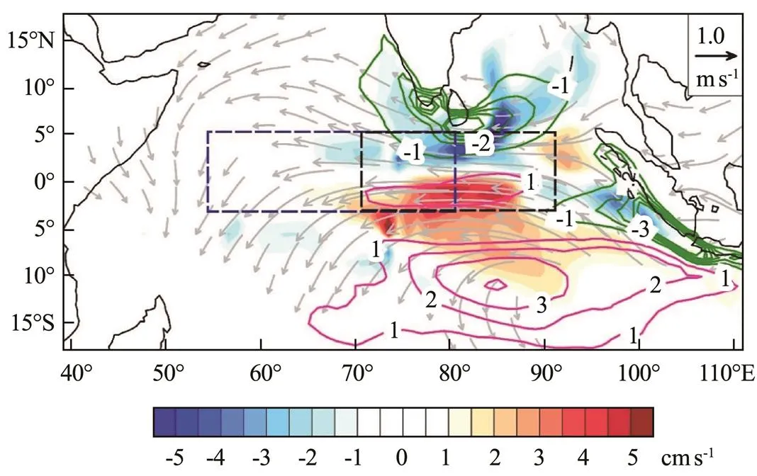
Fig.2 SON wind curl anomaly regressed against PC1 (contour, 10−8Nm−3; only values larger than 1.0×10−8Nm−3 are shown), composite anomalous wind stress (vectors, ms−1), and Va (shading, cms−1) in the subsurface layer (depth=90m) during IOD peak. The red (green) line indicates positive (negative) values. Blue and black dashed rectangles respectively represent regions of meridional divergence in the surface layer (55˚–80˚E) and convergence in the subsurface layer (70˚–90˚E). The composite wind vectors and Va are, according to the Student’s t-test, significant at the 95% confidence level.

Fig.3 Composite anomalous zonal currents (ms−1) in the equatorial region (2.5˚S–2.5˚N) during positive IOD peak season.

Fig.4 (a) Time series of SON volume transport (1Sv=1.0×106m3s−1)bymeridionaldivergence(blueline)andanom- alous equatorial zonal current (red line) in the surface layer from 1958 to 2017. (b) Same as (a), but for the convergence (blue line) and EUC variability (red line) in the subsurface layer. The gray line in (a) and (b) is the DMI (℃) averaged during SON. The correlation coefficient between divergence (convergence) and the anomalous equatorial current in the surface (subsurface) layer is 0.85 (0.53), which is significant at the 95% confidence level.

The meridional divergence and the anomalous equatorial zonal currents in the surface layer are negatively correlated with the DMI during SON, with the correlation coefficients being −0.73 and −0.71 (>95% significance), respectively. This result indicates that the IOD dominates interannual variations in the surface layer (Fig.4a). Moreover, the divergence is positively correlated with anomalous surface equatorial zonal currents, with the correlation coefficient being 0.84 (>95% significance). This result suggests that the weakening of the WJ during the IOD peak can be largely explained by meridional divergence. Furthermore, the divergence decreases the sea surface height in the western basin, and the resulting condition is foundtofavoraweakenedWJ.Moreover,anomalouswest- ward flows north of 7˚S weaken the climatological eastward flows and basin-scale water and heat exchange, thereby sustaining the zonal temperature gradient during the IOD peak (Figs.5a, b). Similarly, the correlations between convergence in the subsurface layer and the EUC variability with the DMI are 0.82 and 0.62 (>95% significance), respectively (Fig.4b). These results suggest that the IOD can also influence subsurface oceanic processes. The convergence is positively correlated with EUC variability as well, with the correlation coefficient being 0.53 (>95% significance). This result implies that the enhancement of the EUC during the IOD peak is largely due to the meridional convergence. More importantly, the enhanced EUC extends to the eastern basin and transports more subsurface water along the equator and Sumatra-Java coast to support the eastern TIO upwelling (Fig.5d). Owing to the strong anticyclonic and cyclonic circulation in the subsurface, meridional convergence occurs in the far north of the anomalous wind stress curl center in the Southern Hemi- sphere, which is different from that in the Northern Hemi- sphere (Fig.2). Scatter diagrams based on 12 chosen IOD events and the spatial regression of equatorial zonal and meridional currents are also derived. The results support the robust relationship between the equatorial zonal and meridional currents (figure not shown).

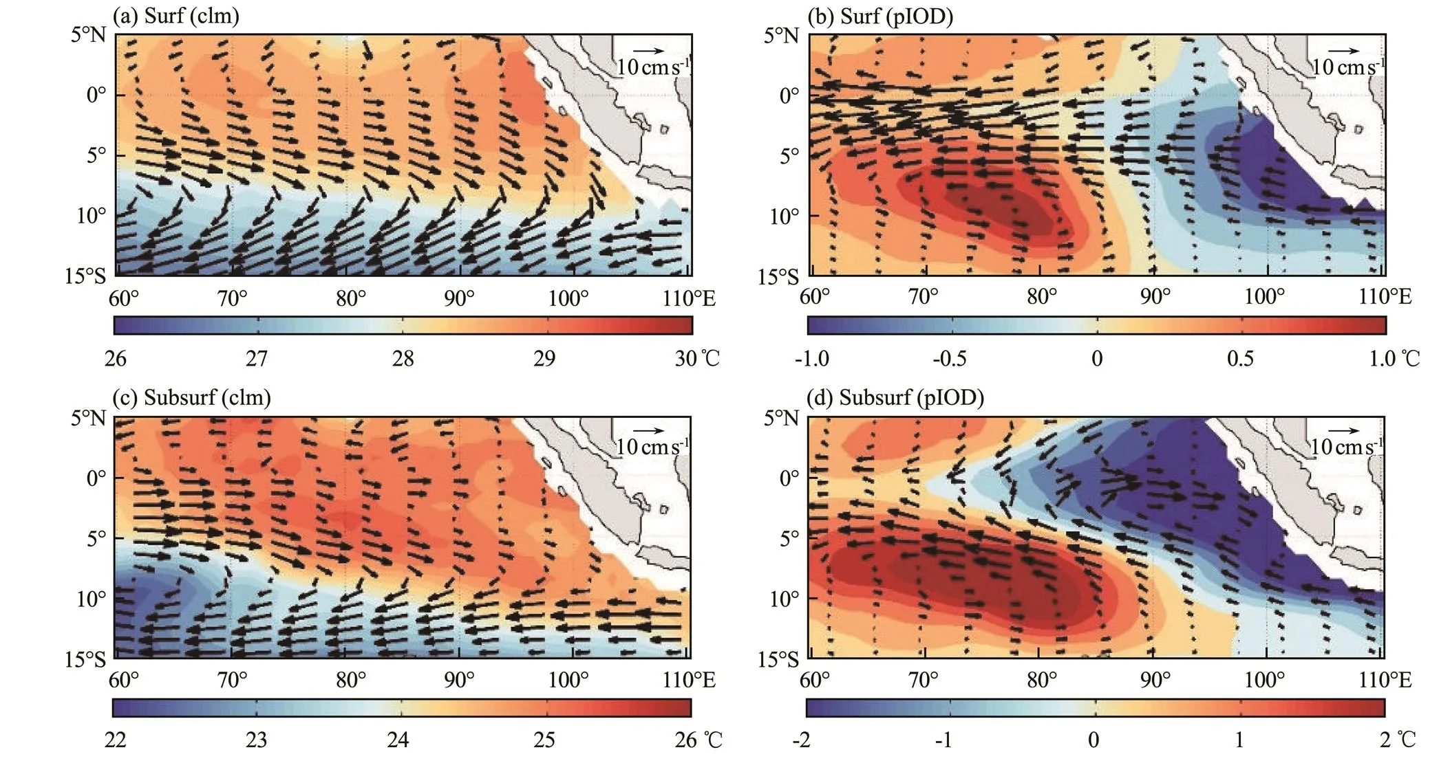
Fig.5 SON composite horizontal currents (vectors, cms−1) and ocean temperature (shading, ℃) in the surface (a) and subsurface (c) layer for the climatological mean state. (b, d) Same as (a, c), but for their anomalies during positive IOD events.

In summary, meridional divergence and convergence are found to favor a weakened WJ in the surface layer and an enhanced EUC in the subsurface layer, respectively. The combined oceanic processes mentioned above indicate novel positive feedback to the IOD, in which the drained and weakened WJ favored by meridional divergence and the strengthened and extended EUC resulting from convergence help sustain the zonal temperature gradient in the TIO. Moreover, the correlation coefficient between convergence and the EUC is somewhat lower than that between divergence and the WJ. This result may be explained by the complexity of the EUC. The EUC is controlled by the zonal pressure gradient in response to equatorial zonal winds and meridional convergence resulting from off-equatorial wind curl anomalies; however, the WJ is controlled only by equatorial zonal winds (Chen, 2016b, 2018).

Three datasets (ECCO2, SODA3.4.2, and CESM outputs) are used to confirm the interannual variability of the meridional currents and their relationship with the equatorial zonal currents. Significant meridional divergence in the surface layer and convergence in the subsurface layer are observed in both hemispheres between 12˚S and 12˚N on the basis of the ECCO2, SODA3.4.2, and CESM outputs (Fig.6a; Fig.7a; Fig.8a); this result is consistent with the ORAS4 results. The explained variances of the main mode are 53.4% for ECCO2, 39.5% for SODA3.4.2, and 64% for CESM. Their dominant patterns are closely related to the IOD as the main principal component (PC1) is highly correlated with the DMI (Fig.6b; Fig.7b; Fig.8b). In addition, the correlation coefficients between meridional divergence (convergence) and the variation of the equatorial zonal current in the surface (subsurface) layer are 0.69 (0.77) for ECCO2, 0.78 (0.61) for SODA3.4.2, and 0.78 (0.85) for CESM (Figs.6c–d; Figs.7c–d; Figs.8c–d). The details of the correlation coefficients are shown in Table 1.

Table 1 Correlation coefficients between SON DMI (℃), PC1, and zonal and meridional transport (Sv) shown in Fig.7, Fig.6, and Fig.8

Notes: PC1 is the main principal component of the EOF analysis. Div represents the meridional divergence in the surface layer, and Conv is the meridional convergence in the subsurface layer. WJ and EUC represent the variations of the equatorial zonal currents in the surface and subsurface layer, respectively. Correlation coefficients exceeding the 99% significance level are shown in bold.

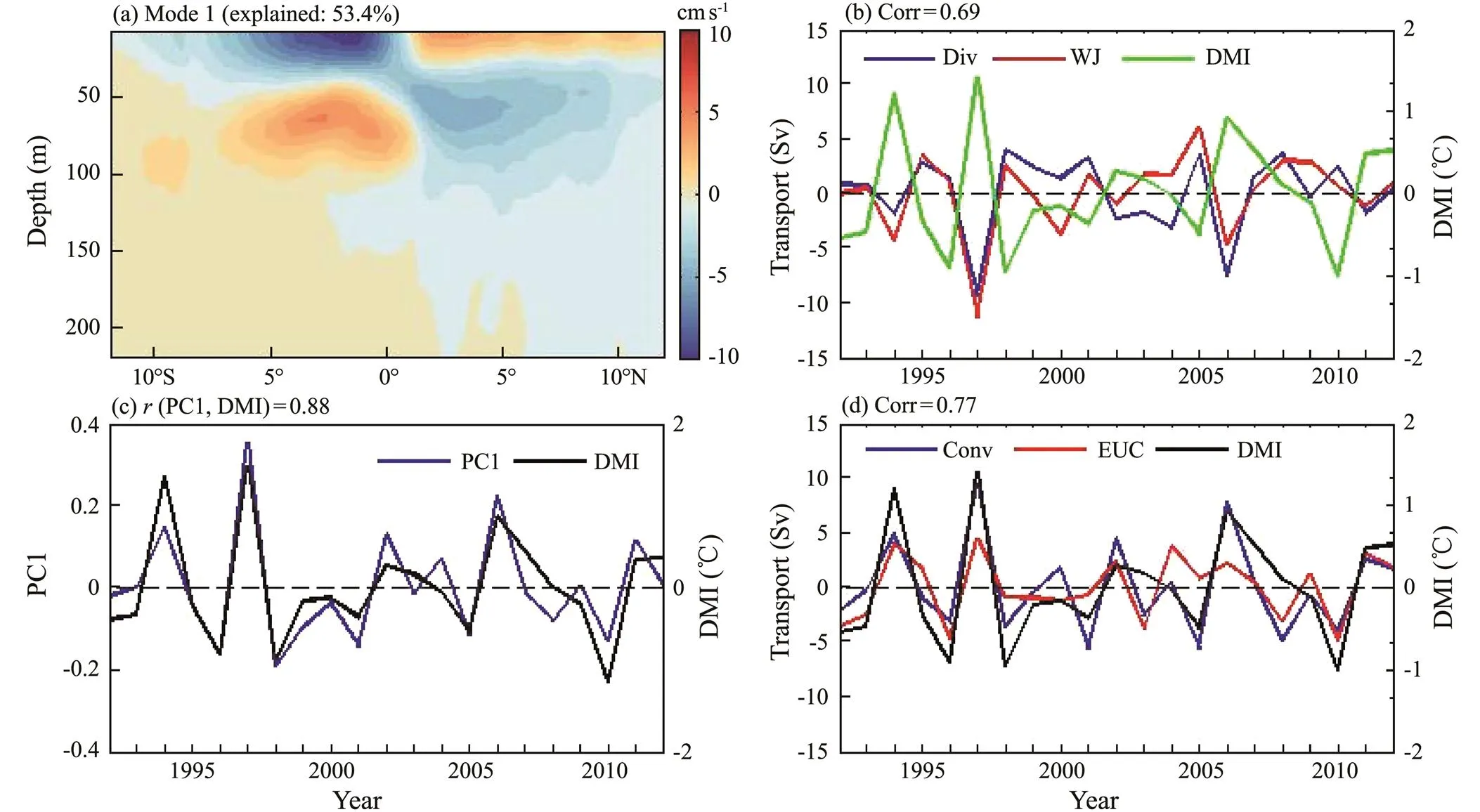
Fig.6 The leading EOF mode (a, cms−1) and corresponding principal component (b, blue line) of zonal-mean (from the western boundary to eastern boundary in the Indian Ocean) meridional current anomalies during SON based on ECCO2. The black line in (b) is the SON DMI calculated according to Saji et al. (1999). The explained variance of the leading mode is 53.4%. The correlation between PC1 and the DMI is 0.88. (c) Time series of SON volume transport anomaly (Sv) by divergence in the surface layer (blue line) and the variations of the WJ (red line). (d) Same as (c), but for the convergence in the subsurface layer (blue line) and the EUC anomaly (red line). The green line in (c) and black line in (d) are the SON DMI (℃). The correlation coefficient of meridional divergence (convergence) and the variation of equatorial zonal currents in the surface (subsurface) layer is 0.69 (0.77), which is significant at the 99% confidence level.

Fig.7 Leading EOF mode (a, cms−1) and corresponding principal component (b, green line) of zonal-mean (from the western boundary to the eastern boundary in the Indian Ocean) meridional current anomalies during SON based on SODA3.4.2. The black line in (b) is the SON DMI (℃) calculated according to Saji et al. (1999). The explained variance of the leading mode is 39.5%. The correlation between PC1 and the DMI is 0.88. (c) Time series of SON volume transport anomaly (Sv) by divergence in the surface layer (blue line) and variations of the WJ (pink line). (d) Same as (c), but for the convergence in the subsurface layer (blue line) and the EUC variability (pink line). The black line in (c) and (d) is the SON DMI (℃). The correlation coefficient of divergence (convergence) and the variations of the equatorial zonal current in the surface (subsurface) layer is 0.78 (0.61), which is significant at the 99% confidence level.

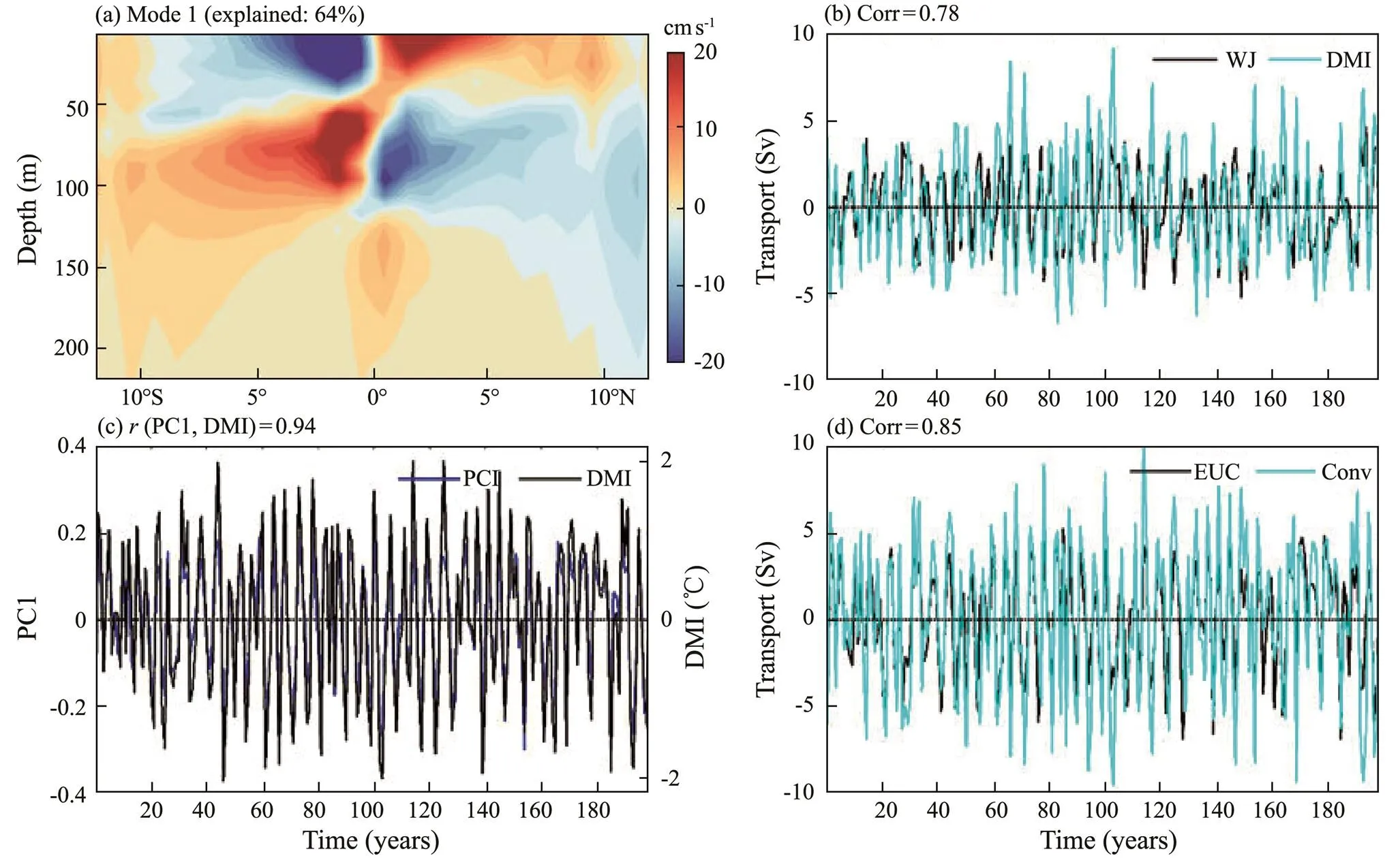
Fig.8 Same as Fig.6, but for the CESM outputs. Notice colors of lines is slightly different from Fig.6 to show contrast of lines more clearly. The explained variance of the leading mode reaches 64% in (a). The correlation between PC1 and the DMI is 0.94 in (b). The correlation coefficient of meridional divergence (convergence) and the variation of equatorial zonal currents in the surface (subsurface) layer is 0.78 (0.85), which is significant at the 99% confidence level.

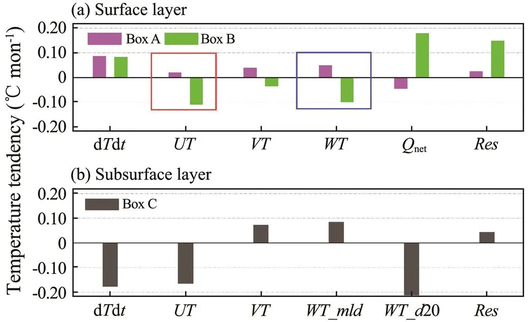
Fig.9 SON mean heat budget terms of the ocean temperature tendency (dTdt); the zonal (UT), meridional (VT), andvertical (WT) advection terms; the net heat flux term (Qnet); and the residual term (Res) in Box A (a, pink bar), Box B (a, green bar), and Box C (b, gray bar). The red and blue boxes highlight the zonal and vertical advection in the surface layer, respectively.

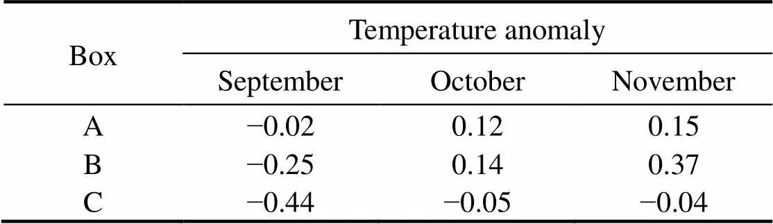
Table 2 Temperature anomaly tendency in Boxes A−C (Unit: ℃mon−1)

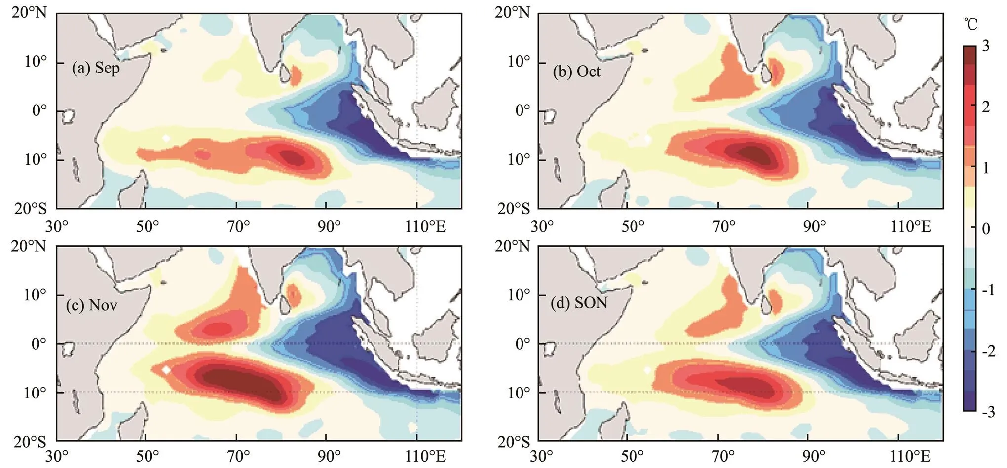
Fig.10 Subsurface ocean temperature anomaly (unit: ℃) during the IOD peak for September (a), October (b), November (c), and SON mean (d) in the TIO.

In addition to supplying the EUC, the convergence could give rise to significant local upwelling at the base of the mixed layer and thus cool the temperature in the equatorial central Indian Ocean (CIO). A cold tongue in the equatorial CIO has consistently been found in response to easterlies as an indicator of equatorial upwelling (Xie, 2002). Simultaneously, upwelling Kelvin waves are induced because of local upwelling. Subsequently, Kelvin waves propagate along the equator until the Sumatra-Java coast and favor local cooling. Using a novel process index regression method, Delman(2018) quantitatively assessed the contribution of equatorial Kelvin waves to eastern Indian Ocean cooling and concluded that their roles are not negligible for IOD growth. Nevertheless, the relative contributions of upwelling Kelvin waves and zonal advection to cooling the SSTA in the eastern basin remain unclear. Thus, a quantitative analysis is needed in a future study.

4 Summary and Discussion

In this study, the monthly model output of the ECMWF ORAS4 from 1958 to 2017 is used to explore the responses of the equatorial ocean currents and their roles in sustaining the zonal temperature gradient during the IOD peak. A novel positive feedback mechanism summarizes the oceanic processes (Fig.11).

Fig.11 Schematic of key oceanic processes during the positive IOD peak. The hollow arrow marks the equatorial easterly wind anomalies. −Curl is the anticyclonic wind stress curl anomaly. The thin gray arrows represent the meridional divergence in the surface layer, and the thin blue arrows represent meridional convergence in the subsurface layer. The wide blue arrows denote the off-equatorial Ekman downwelling and anomalous equatorial CIO upwelling. The black arrows are the anomalous westward current in the surface layer and the enhanced EUC in the equatorial region. The dotted blue line represents the boundary between the surface and subsurface layers.

This study investigates the significant oceanic processes in the TIO in response to surface winds during the IOD peak. On the one hand, anomalous westward surface currents occur in the equatorial region. The WJ weakens substantially, and the drained WJ weakens the eastward water mass and heat exchange. The EUC intensifies, and the enhanced EUC extends to the eastern basin and transports more subsurface water to support upwelling in the eastern Indian Ocean. On the other hand, significant meridional divergence at 55˚–80˚E in the surface layer and convergence at 70˚–90˚E in the subsurface layer are observed (Fig.1). The divergence is caused by the direct Ekman drift and pile-up effects of the anomalous westward surface currents induced by equatorial easterlies, whereas the convergence is caused by equatorward mass transport resulting from Ekman downwelling due to off- equatorial wind curl anomalies (Fig.2). Owing to the strong subsurface anticyclonic and cyclonic circulation in the Southern Hemisphere, the location of meridional convergence does not correspond well with the wind curl center, however, they correspond well in the northern Hemisphere (Fig.5).

The maximum variation regions of the equatorial zonal currents in the surface and subsurface layers correspond well with those of the meridional divergence and convergence, respectively. The meridional divergence and convergence are found to favor a weakened WJ in the surface layer and an enhanced EUC in the subsurface layer, respectively. These ocean responses, therefore, suggest that novel ocean positive feedback maintains zonal temperature gradient during the IOD peak. Specifically, the weakened WJ favored by meridional divergence warms the eastern Indian Ocean, and the enhanced EUC contributed by convergence cools the eastern basin (Figs.4, 5, and 9). Moreover, the positive feedback is novel and slightly different from the Bjerknes feedback. The former highlights the roles of three-dimensional ocean currents in sustaining the IOD peak, whereas the latter emphasizes the roles of zonal SSTA, winds, and thermocline, all of which are responsible for IOD evolution.

Many studies have noted the oceanic processes during the IOD peak. However, the relation between equatorial zonal and meridional currents and their roles in the IOD have not been fully investigated. Sun(2014) pointed out the meridional divergence in the mixed layer but failed to examine the related feedback mechanism to the IOD. Using observational data, Zhang. (2014) and McPhaden(2015) studied the contributions of equatorial zonal currents to the IOD and briefly examined the linkages between meridional transport and equatorial zonal currents. However, they used only onemeasurement at 0˚, 80.5˚E to represent the equatorial zonal current in their studies. Such application is insufficient to produce a full picture of spatial variations. In the current study, additional details are investigated, and the dynamic linkages between them are explored through statistical analysis and temperature heat budget analyses (Figs.5 and 9). The novel positive feedback provides new insights into the IOD dynamics and may be used to refine ocean models for simulation and prediction.

The dynamics of this novel positive feedback mechanism to the IOD is somewhat consistent with the recharge oscillator theory, delayed oscillator theory, and advective-reflective oscillator theory for ENSO in the Pacific Ocean (Jin, 1997; Picaut, 1997; Kang and An, 1998; Suarez and Schopf, 1988; An and Kang, 2000). First, ocean dynamics in the positive feedback plays a role in recharging the IOD through the connections between meridional divergence and convergence with equatorial zonal currents in the surface and subsurface layer, respectively. Second, significant anomalous upwelling in the equatorial CIO due to subsurface convergence cools the local temperature and induces upwelling Kelvin waves. The upwelling waves further cool the surface temperature in the eastern basin upon arrival. This process is similar to delayed oscillator theory during the establishment of La Niña (Suarez and Schopf, 1988). Third, zonal advection in the equatorial region has a major contribution to the development of the IOD, similar to the advective-reflective oscillator proposed by Picaut(1997). However, owing to the differences in the mean state between these two oceans, we do not have comprehensive knowledge of the ocean dynamics in the Indian Ocean in relation to the three theories.

Finally, a similar analysis is performed for negative IOD events. In some strong negative IOD years (such as 1996, 1998, and 2010), similar ocean processes exist. Nevertheless, the composite of negative IOD events does not effectively capture the ocean processes when all negative IOD events are considered. This result is due to the asymmetry of the positive and negative IOD events that has been noted in many studies (, Ummenhofer, 2013; Wang, 2014). Therefore, the results presented in the current work mainly pertain to positive IOD events.

Acknowledgements

The ECMWF ORAS4 reanalysis data were downloadedfrom http://apdrc.soest.hawaii.edu/dods/public_data/Reanal-ysis_Data/ORAS4. This work was supported by the National Key R&D Program of China (No. 2019YFA0606701), the Strategic Priority Research Program of the Chinese Academy of Sciences (No. XDA20060502), the National Natural Science Foundation of China (Nos. 42076020, 41776023 and 91958202), the Key Special Project for Introduced Talents Team of Southern Marine Science and Engineering Guangdong Laboratory (Guangzhou) (No. GML2019ZD0306), the Innovation Academy of South China Sea Ecology and Environmental Engineering of the Chinese Academy of Sciences (No. ISEE2018PY06), the Key Research Program of the Chinese Academy of Sciences (No. ZDRW-XH-2019-2), the Youth Innovation Promotion Association of the Chinese Academy of Sciences (No. 2020340), the Rising Star Foundation of the SCSIO (No. NHXX2018WL0201), and the Independent Research Project Program of the State Key Laboratory of Tropical Oceanography (No. LTOZZ2101). The authors also gratefully acknowledge the use of the HPCC for all numeric simulations and data analysis at the South China Sea Institute of Oceanology, Chinese Academy of Sciences.

An, S., and Kang, I., 2000. A further investigation of the recharge oscillator paradigm for ENSO using a simple coupled model with the zonal mean and eddy separated., 13: 1987-1993.

Balmaseda, M. A., Mogensen, K., and Weaver, A., 2013. Evaluation of the ECMWF ocean reanalysis ORAS4., 139: 1132-1161, DOI: 10.1002/qj.2063.

Bjerknes, J., 1969. Atmospheric teleconnections from the equatorial Pacific., 97 (3): 163-172.

Carton, J. A., Chepurin, G. A., and Chen, L., 2018. SODA3: A new ocean climate reanalysis., 31: 6967-6983, DOI: 10.1175/JCLI-D-18-0149.1.

Chen, G., Han, W., Li, Y., Wang, D., and McPhaden, M. J., 2015. Seasonal-to-interannual time-scale dynamics of the equatorial undercurrent in the Indian Ocean.,45: 1532-1553, DOI: 10.1175/JPO-D-14-0225.1.

Chen, G., Han, W., Shu, Y., Li, Y., Wang, D., and Xie, Q., 2016a. The role of equatorial undercurrent in sustaining the eastern Indian Ocean upwelling., 43: 6444-6451, DOI: 10.1002/2016GL069433.

Chen, H., Hu, Z., Huang, B., and Sui, C., 2016b. The role of reversed equatorial zonal transport in terminating an ENSO event., 29 (16): 5859-5877, DOI: 10.1175/JCLI-D-16-0047.1.

Chen, H., Sui, C., Tseng, Y., and Huang, B., 2018. Combined role of high- and low-frequency processes of equatorial zonal transport in terminating an ENSO event., 31: 5461-5483, DOI: 10.1175/JCLI-D-17-0329.1.

Chowdary, J. S., and Gnanaseelan, C., 2007. Basin-wide warming of the Indian Ocean during El Niño and Indian Ocean Dipole years., 27 (11): 1421-1438.

de Boyer Montégut, C., Madec, G., Fischer, A. S., Lazar, A., and Iudicone, D., 2004. Mixed layer depth over the global ocean: An examination of profile data and a profile-based climatology., 109: C12003.

Dee, D. P., Uppala, S. M., Simmons, A. J., Berrisford, P., Poli, P., Kobayashi, S.,, 2011. The ERA-Interim Reanalysis: Configuration and performance of the data assimilation system., 137: 553-597.

Delman, A. S., McClean, J. L., Sprintall, J., Talley, L. D., and Bryan, F. O., 2018. Process-specific contributions to anomalous Java mixed layer cooling during positive IOD events., 123: 4153-4176, DOI: 10.1029/-2017JC013749.

Delman, A. S., Sprintall, J., McClean, J. L., and Talley, L. D., 2016. Anomalous Java cooling at the initiation of positive Indian Ocean Dipole events., 121: 5805-5824.

Feng, M., and Meyers, G., 2003. Interannual variability in the tropical Indian Ocean: A two‐year time‐scale of Indian Ocean Dipole., 50: 2263-2284.

Gnanaseelan, C., and Deshpande, A., 2018. Equatorial Indian Ocean subsurface current variability in an Ocean General Circulation Model., 50: 1705-1717.

Gnanaseelan, C., Deshpande, A., and McPhaden, M. J., 2012. Impact of Indian Ocean Dipole and El Niño/Southern Oscillation wind-forcing on the Wyrtki jets., 117: C08005, DOI: 10.1029/2012JC007918.

Huang, B., and Kinter III, J. L., 2002. Interannual variability in the tropical Indian Ocean., 107 (C11): 3199, DOI: 10.1029/2001JC001278.

Hurrell, J. W., Holland, M. M., Gent, P. R., Ghan, S., Kay, J. E., Kushner, P. J.,, 2013. The community earth system model: A framework for collaborative research., 94 (9): 1339-1360.

Iskandar, I., Masumoto, Y., and Mizuno, K., 2009. Subsurface equatorial zonal current in the eastern Indian Ocean., 114: C06005, DOI: 10.1029/2008JC005188.

Jin, F. F., 1997. An equatorial ocean recharge paradigm for ENSO. Part I: Conceptual model., 54: 811-829.

Kang, I., and An, S., 1998. Kelvin and Rossby wave contributions to the SST oscillation of ENSO., 11: 2461-2469.

Karmakar, A., Parekh, A., Chowdary, J. S., and Gnanaseelan, C., 2017. Inter comparison of tropical Indian Ocean features in different ocean reanalysis products., 51: 119-141, DOI: 10.1007/s00382-017-3910-8.

Knauss, J. A., and Taft, B. A., 1964. Equatorial undercurrent of the Indian Ocean., 143 (3604): 354-356.

Krishnan, R., and Swapna, P., 2009. Significant influence of the boreal summer monsoon flow on the Indian Ocean response during dipole events., 22 (21): 5611-5634.

Li, T., Wang, B., Chang, C. P., and Zhang, Y., 2003. A theory for the Indian Ocean Dipole Mode–Zonal mode., 60: 2119-2135.

Madec, G., 2008. NEMO ocean engine.No. 27, 1-391.

McPhaden, M. J., Wang, Y., and Ravichandran, M., 2015. Volume transports of the Wyrtki jets and their relationship to the Indian Ocean Dipole., 120: 5302-5317, DOI: 10.1002/2015JC010901.

Nagura, M., and McPhaden, M. J., 2008. The dynamics of zonal current variations in the central equatorial Indian Ocean., 35 (23): 186-203, DOI: 10.1029/2008-GL035961.

Nagura, M., and McPhaden, M. J., 2010. Dynamics of zonal current variations associated with the Indian Ocean Dipole., 115: C11026, DOI: 10.1029/2010JC-006423.

Nagura, M., and McPhaden, M. J., 2016. Zonal propagation of near surface zonal currents in relation to surface wind forcing in the equatorial Indian Ocean., 46 (12): 3623-3638.

Nyadjro, E. S., and McPhaden, M. J., 2014. Variability of zonal currents in the eastern equatorial Indian Ocean on seasonal to interannual time scales., 119: 7969-7986, DOI: 10.1002/2014JC010380.

Picaut, J., Masia, F., and du Penhoat, Y., 1997. An advective-reflective conceptual model for the oscillatory nature of the ENSO., 277: 663-666.

Rao, R. R., Horii, T., Masumoto, Y., and Mizuno, K., 2017a. Observed variability in the upper layers at the equator, 90˚E in the Indian Ocean during 2001–2008, 1: Zonal currents., 49 (3): 1077-1105.

Rao, R. R., Horii, T., Masumoto, Y., and Mizuno, K., 2017b. Observed variability in the upper layers at the Equator, 90˚E in the Indian Ocean during 2001–2008, 2: Meridional currents., 49 (3): 1031-1048.

Rao, S. A., and Behera, S. K., 2005. Subsurface influence on SST in the tropical Indian Ocean: Structure and interannual variability., 39 (1-2): 103-135.

Rao, S. A., Behera, S. K., and Masumoto, Y., 2002. Interannual subsurface variability in the tropical Indian Ocean with a special emphasis on the Indian Ocean Dipole., 49: 1549-1572.

Reppin, J., Schott, F. A., Fischer, J., and Quadfasel, D., 1999. Equatorial currents and transports in the upper central Indian Ocean: Annual cycle and interannual variability., 104 (C7): 15495-15514, DOI: 10.1029/1999JC900093.

Sachidanandan, C., Lengaigne, M., Muraleedharan, P. M., and Mathew, B., 2017. Interannual variability of zonal currents in the equatorial Indian Ocean: Respective control of IOD and ENSO., 67 (7): 857-873.

Saji, N. H., 2018. The Indian Ocean Dipole.. Oxford University Press, Oxford, 1-34, DOI: 10.1093/acrefore/9780190228620.013.619.

Saji, N. H., Goswami, B. N., Vinayachandran, P. N., and Yamagata, T., 1999. A dipole mode in the tropical Indian Ocean., 401 (6751): 360-363.

Smith, R., Jones, P., Briegleb, B., Bryan, F., Danabasoglu, G., Dennis, J.,, 2010. The parallel ocean program (POP) reference manual: Ocean component of the community climate systemmodel (CCSM) and community earth system model (CESM). LAUR-01853, 141: 1-140.

Suarez, M. J., and Schopf, P. S., 1988. A delayed action oscillator for ENSO., 45 (21): 3283-3287.

Sun, S., Fang, Y., Feng, L., and Tana, 2014. Influence of the Indian Ocean Dipole on the Indian Ocean meridional heat trans- port., 134: 81-88, DOI: 10.1016/j.jmarsys.2014.02.01.

Ummenhofer, C. C., Schwarzkopf, F. U., Meyers, G., Behrens, E., Biastoch, A., and Böning, C. W., 2013. Pacific Ocean contribution to the asymmetry in eastern Indian Ocean variability., 26: 1152-1171.

Uppala, S. M., KÅllberg, P. W., Simmons, A. J., Andrae, U., Da Costa Bechtold, V., Fiorino, M.,, 2005. The ERA-40 re-analysis., 131: 2961-3012, DOI: 10.1256/qj.04.176.

Vinayachandran, P. N., Saji, N. H., and Yamagata, T., 1999. Response of the equatorial Indian Ocean to an anomalous wind event during 1994., 26 (11): 1613-1615.

Wang, W., Zhu, X., Wang, C., and Köhl, A., 2014. Deep meridional overturning circulation in the Indian Ocean and its relation to Indian Ocean Dipole., 27: 4508-4520.

Webster, P. J., Moore, A. M., Loschnigg, J. P., and Leben, R. R., 1999. Coupled ocean-atmosphere dynamics in the Indian Ocean during 1997–98., 401 (6751): 356-360.

Wyrtki, K., 1973. An equatorial jet in the Indian Ocean., 181 (4096): 262-264.

Xie, S.-P., and Philander, S. G. H., 1994. A coupled ocean-atmosphere model of relevance to the ITCZ in the eastern Pacific., 46 (4): 340-350.

Xie, S.-P., Annamalai, H., Schott, F. A., and McCreary, J. P., 2002. Structure and mechanisms of South Indian Ocean climate variability., 15 (8): 864-878.

Yamagata, T., Behera, S. K., Luo, J. J., Masson, S., and Jury, M. R., 2004. Coupled ocean-atmosphere variability in the tropical Indian Ocean. In:. Wang, C. Z.,, eds., Geophysical Monograph Series, AGU, Washington DC, 147: 189-212.

Yu, W., Xiang, B., Liu, L., and Liu, N., 2005. Understanding the origins of interannual thermocline variations in the tropical Indian Ocean., 32: L24706, DOI: 10.1029/2005GL024327.

Zhang, D., McPhaden, M. J., and Lee, T., 2014. Observed interannual variability of zonal currents in the equatorial Indian Ocean thermocline and their relation to Indian Ocean Dipole., 41: 7933-7941.

Zhang, R., Wang, X., and Wang, C. Z., 2018. On the simulations of global oceanic latent heat flux in the CMIP5 multimodel ensemble., 31: 7111-7128, DOI: 0.1175/JCLI-D-17-0713.1.

(Oceanic and Coastal Sea Research)

https://doi.org/10.1007/s11802-022-4864-y

ISSN 1672-5182, 2022 21 (3): 622-632

(December 3, 2020;

February 4, 2021;

April 14, 2021)

© Ocean University of China, Science Press and Springer-Verlag GmbH Germany 2022

Corresponding author. E-mail: weiqiang.wang@scsio.ac.cn

(Edited by Xie Jun)