
Groove modeling and digital simulation for intersecting structures of circular tubes based on coplanarity of vectors
2022-07-26 08:18ChenChangrongZhouSunshengLianGuofuHuangXuFengMeiyanGaoXianfeng
China Welding 2022年2期
Chen Changrong , Zhou Sunsheng , Lian Guofu , Huang Xu , Feng Meiyan , Gao Xianfeng
1. School of Mechanical and Automotive Engineering, Fujian University of Technology, Fuzhou 350118, China;2. Fujian Fuchuan Yifan New Energy Equipment Manufacturing Co., Ltd., Zhangzhou 363211, China
Abstract In order to establish the groove model for intersecting structures of circular tubes, mathematical model of the intersecting line is established by the method of analytic geometry, and parametric equations are thus determined. The dihedral angle, groove angle and actual cutting angle for any position of the intersecting line are derived as well. In order to identify groove vectors for two pipes, a new analytical method, i.e. coplanarity of vectors, is further proposed to complete the groove model. The established model is virtually verified by programming and simulation calculation in the MATLAB environment. The results show that groove vectors of intersecting structures simulated by MATLAB are consistent with the theoretical groove model, indicating that the theoretical groove model established in this paper is accurate,and further proves that the proposed coplanarity of vectors for solving groove vectors is correct and feasible. Finally, a graphical user interface (GUI) is developed by MATLAB software to independently realize functions such as model drawing, variable calculation and data output. The research outcome provides a theoretical foundation for the actual welding of circular intersecting structures, and lays an essential basis for weld bead layout and path planning.
Key words method of analytic geometry in space, intersecting line mathematical model, coplanarity of vectors, groove model, MATLAB simulation
0 Introduction
The offshore operation platform, an important facility that works through the whole process of marine resource development, is complex in structure and mainly composed of multiple sets of jacket intersecting structures[1 – 4]. The biggest difficulty in building an offshore platform lies in the jacket combination, which in turn depends on the construction of intersecting structures, specifically the modelling of groove at both intersected pipes. Therefore, solving the groove vector accurately is the basis for constructing and realizing the marine operation platform.
Many scholars have done corresponding research on the groove modeling of circular intersecting structures. Zhao et al[5]analyzed the mathematical constraint model required for cutting intersecting structures of circular tubes, and proposed a method to solve the trajectory of intersecting line by coordinate transformation and parametric equations. Based on the established mathematical model of the intersecting line the groove vector of the branch pipe can be used to conveniently control the position and attitude of the cutting torch. The issue is that this study did not solve the main groove vector but approximated it as a plane. This approach is inaccurate because the surface of the main pipe groove vector is actually a curved surface with a certain curvature-an approximate elliptical surface[6]. Miao[7]studied the intersecting structure of circular tubes, and established the cutting mathematical model of the groove with a new calculation method. The fixed-angle groove and fixedpoint groove vectors were thus calculated. This study did not solve the main groove vector, and the established intersecting line groove model was not accurate enough, either.Wang et al.[8]established a general mathematical model of circular intersecting structure, deduced the mathematical equation of the intersecting line using the spatial analytic geometry theory, and presented corresponding parametric equation. However, the groove model was not established for the intersecting structure. Wang et al.[9]established a mathematical model for the intersected circular tubes according to the principle of spatial analytic geometry, and proposed a solution for the groove vector. This study did not solve the groove vector for the main pipe, still. Song et al.[10]calculated the welding groove model of intersecting pipes and established the mathematical model of the groove,including the groove angle and the spatial curve of the intersecting line. The research did not solve the groove vector of the main pipe and the branch pipe, but generated the groove model by fitting in the 3D software SolidWorks, and the established groove model was not accurate enough. Liu et al.[11]established an ideal intersecting line model, expressed it with parametric equations, and further combined the inherent characteristics of the intersecting line to model the intersecting structure in the actual welding process.However, the research did not fully establish the groove model of the intersecting line.
From literature reviewed, the current research on the groove of circular intersecting structures is still mainly focused on establishment of mathematical models of the intersecting line and the groove vector of branch pipe, while the groove vector of the main pipe is approximated to a plane.This simplification is different from the actual pipe groove which is composed of curved ellipsoid surface.
In this paper, a novel method for modeling grooves of circular intersecting structures is proposed based on the coplanarity of vectors. Firstly, the mathematical model of the intersecting line is established by the spatial analysis method, and then the parametric equation of the intersecting line is given. With the mathematical model of the intersecting line, the dihedral angle, groove angle, and actual cutting angle of the intersecting structure are solved. The coplanar method is used to solve the groove vector for both the main pipe and the branch pipe. Finally, the calculation and simulation of the groove model are carried out within MATLAB and the graphical user interface is developed, which proves that the proposed method for solving the groove model is feasible and accurate. The research results provide a theoretical basis for the actual welding of the jacket intersecting structure, and lay a solid foundation for groove bead layout and path planning.
1 Mathematical model of intersecting line
1.1 Establishment of the coordinate system
Let the radii of the main pipe and the branch pipe beRandr, respectively (whereR>r). The axes of two circular tubes have a distance ofe(whene= 0, two axes are coplanar), the included angle isα, and intersect with the common perpendicular line atOandO1, respectively. The main pipe coordinate systemO-XYZand the branch pipe coordinate systemO1-X1Y1Z1are both right-hand Cartesian coordinate systems.
TheO-XYZcoordinate system of the main pipe takesOas the origin. The axis of the main pipe is theYaxis. The axis perpendicular to theYaxis andOO1is theZaxis, and theXaxis is determined by the right-hand rule, as shown in Fig. 1.
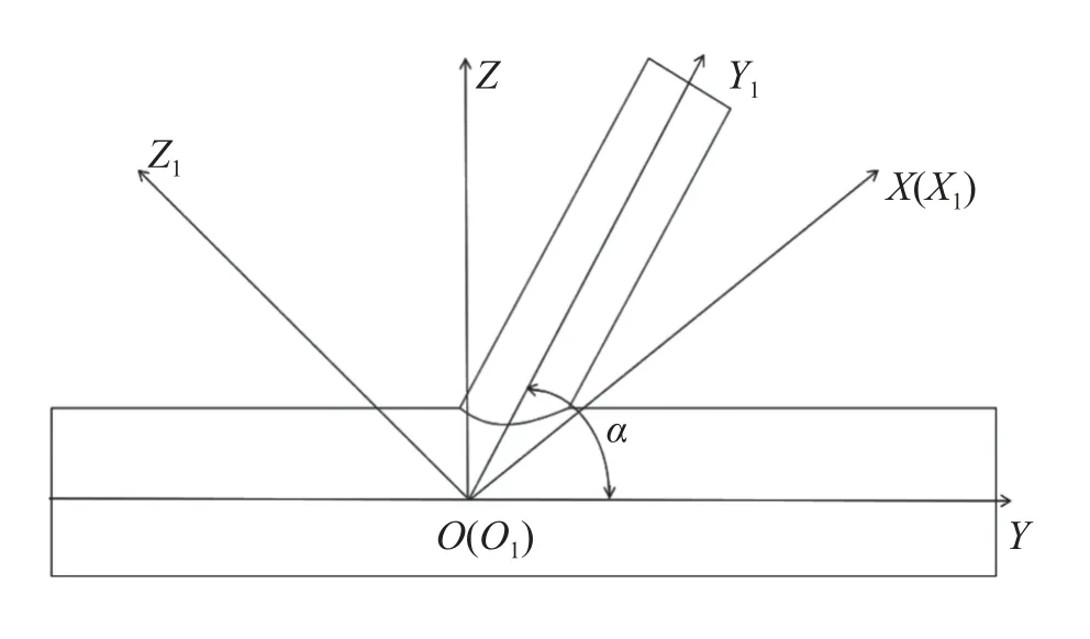
Fig.1 Schematic diagram of the coordinate systems for intersecting circular tubes
Similarly, theO1-X1Y1Z1coordinate system of the branch pipe takesO1as the origin. The axis of the branch pipe is theY1axis. The axis perpendicular to theY1axis and theOO1is theZ1axis. TheX1axis is coaxial to theXaxis[12].
1.2 Transformation of coordinate system and solution of intersecting line
Rotating theO-XYZcoordinate system counterclockwise around theXaxis byαand offsettingeyields theO1-X1Y1Z1[13 – 14]. The conversion relationship of the rotation transformation is
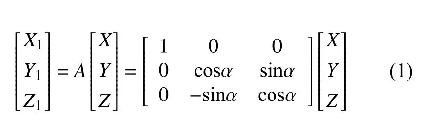
whereAis the rotation matrix of theO-XYZcoordinate system rotating counterclockwise around theX-axis to theO1-X1Y1Z1coordinate system. Based on Equation (1), the relationship between two coordinate systems is
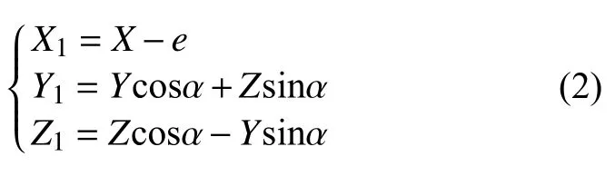
Similarly, the transformation relationship from theO1-X1Y1Z1coordinate system to theO-XYZcoordinate system is as follows:

In theO-XYZcoordinate system, the equation of the main pipe is

InO1-X1Y1Z1, the equation of the branch pipe is
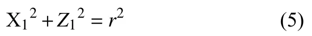
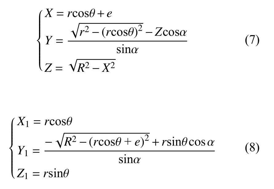
Projecting any weld point (X1,Y1,Z1) on the branch pipe into theO1-X1Z1plane coordinates, and setting its polar coordinates as (r,θ), then the parametric equation is obtained as follow:
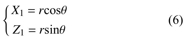
By solving Eq. (2), (4), (5) and (6) simultaneously, the equation of the intersecting line in two coordinate systemO-XYZcan be derived as Eq.s (7) and (8) , respectively:
2 Dihedral angle,groove angle and actual cutting angle
According to the welding code (AWS or API), the groove angle is determined by the dihedral angle which is the angle between tangent planes of two cylindrical surfaces passing through the intersecting point. The dihedral angles at different points on the intersecting line are different and vary with the phase angle[15]. Therefore, the premise of determining the groove angle is to calculate the dihedral angle.
In Fig. 2, φ is the dihedral angle of a point on the intersecting line, i.e. the angle between the main pipe tangent planeQmand the branch pipe tangent planeQbof the intersecting structure.npis the groove vector of the branch pipe,where the cutting torch positions. The angle between the vectornpand the planeQbis the theoretical cutting angle ω of the groove. The angle between the vectornpand the tangent planeQmis the groove angle ϕ. β is the actual cutting angle of the groove.
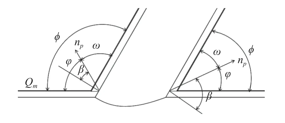
Fig.2 Relationship between dihedral angle,actual cutting angle and groove angle
Fig. 3 is a schematic diagram of each vector at the groove.ngis the vector of any point at the groove of the main pipe, whereng0andng1are the groove vectors of the main pipe at the initial point and the end point, respectively.nmandnbare the unit normal vectors of tangent planesQmandQb, respectively. The angle betweennmandnpisμ, and the angle betweennbandnpisσ. The relationships are:µ=90◦−ϕ、σ=90◦−ω.
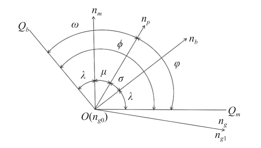
Fig.3 Schematic diagram of vectors relating to the groove
2.1 Solution of dihedral angle
From Eq. (4) and Eq. (5) in Section 1.2, it can be known that the unit normal vectors of the tangent planesnmandnbat any point on the intersecting line can be obtained in their respective coordinate systems as follows:
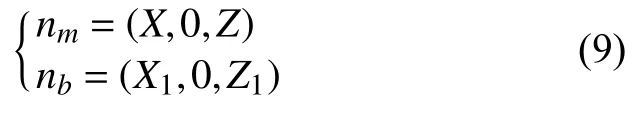
Applying Eq. (3) and Eq. (7) in Section 1.2,nbcan be converted to the main coordinate system as
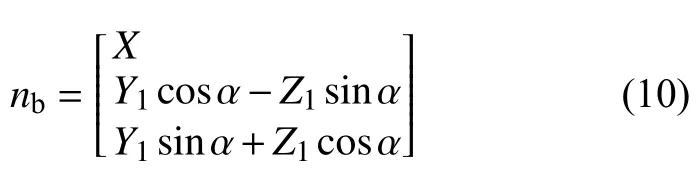
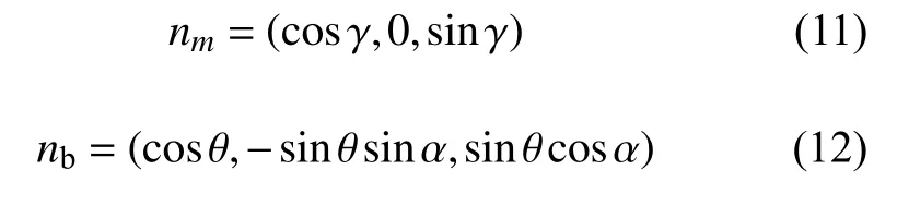
X1=rcosθ,Z1=rsinθ,X=Rcosγ,Z=Rsinγ, whereγis the position angle in the main coordinate system. Therefore, the unit normal vectornmof the main tangent plane and the unit normal vectornbof the branch tangent plane can be written as
According to the cosine formula of the two-unit normal vector:
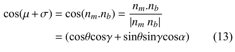
whereγis

It can be seen that the dihedral angle φ is
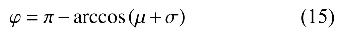
2.2 Solution of groove angle
According to the American Petroleum Institute standard,when the dihedral angle φ ≥90◦, the groove angle ϕ=45◦;when the dihedral angle φ<90◦, groove angle ϕ=φ/3,namely
2.3 Solution of the actual cutting angle
The relationship between the dihedral angle, the groove angle and the actual cutting angle can be observed from Fig. 2.Then, the actual cutting angle β is

3 Solution of groove Vector
3.1 Groove vector for the branch pipe
3.1.1 Traditional solution methods
After establishing the mathematical model of the intersecting line, and calculating the dihedral angle, groove angle, and actual cutting angle at the intersecting position, it is still necessary to solve the groove vector according to the requirements of the welding groove[6].
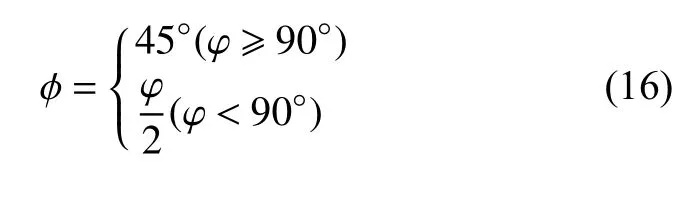
The angle µ between the vectorsnmandnpand the angle σ between thenpandnb, from Fig. 3, conform to the conditions: µ=90◦−ϕ、σ=90◦−ω. Assuming that the groove vector isnp=(1,bp,cp), the following equations can be derived as
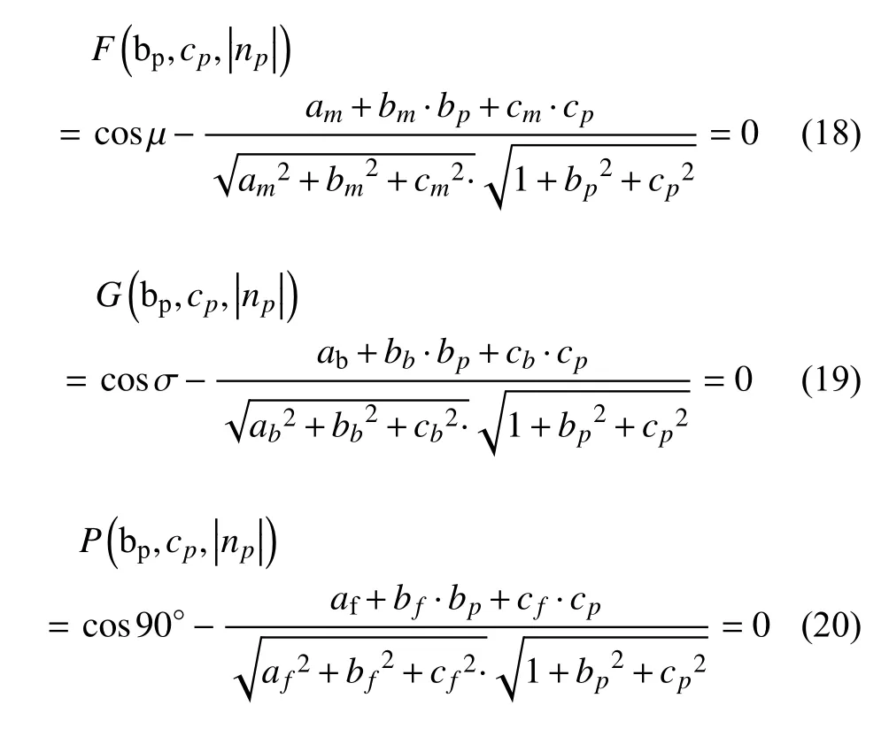
where the direction vector (the vector perpendicular to the normal vector of the main pipe and the branch pipe)[6]nfis
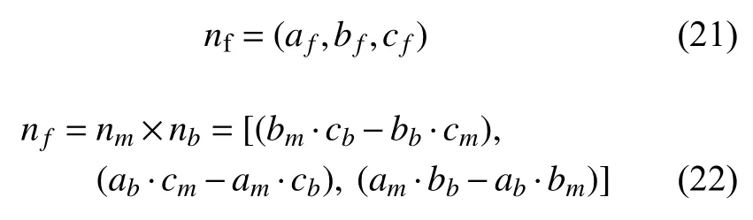
i.e.

From Eq.s (18), (19) and (20),bp,cpandnpcan be resolved. In this way, the equation of a line with the direction vectornppassing through a certain point (X0,Y0,Z0) is
3.1.2 Coplanarity of vectors
It can be seen from Section 3.1.1 that the traditional solution method to the groove vector involves the following procedure: firstly, the direction vectornfshould be obtained by means of the normal vectorsnmandnb, and thenbpandcpcan be obtained according to the equation system,leading to the groove vectornp. The direction ofnpfor a certain point (X0,Y0,Z0) on the intersecting line is lastly calculated by the straight line equation. The calculation process is complicated and tedious. Not only need the direction vectornfbe solved, but also the groove vector at a specific point on the intersecting line. Using coplanarity of vectors to solve the groove vector can simplify the complex and tedious calculation process.
From Fig. 3, the three vectorsnm,nb, andnpare coplanar. Therefore, the branch groove vectornpcan be represented by the normal vectorsnmandnb, namely

Projecting the vectorsnmandnbonto the branch groove vectornpyields the following relationship

The simultaneous Eq.s (27), (28) and (29) are
At this time, it is only necessary to solveaandb, and the vectornpcan be represented by the known vectorsnmandnb. The proposed method is more convenient than the traditional solution. It avoids solving the direction vectornf,the direction of groove vector, which simplifies the complex and tedious formula calculation.
3.2 The main groove vector
According to the method proposed in Section 3.1.2, the groove vector for the main pipe of the intersecting structure can be obtained similarly. According to Fig. 3, the vectorsnm,nb, andngare also coplanar, thus
Assuming that the position angle of the end point ofngat the main pipe isγ1, and the position angle of the starting point isγ0. The coordinates of the groove vectorngat the end point can be expressed as
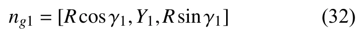
Similarly, the coordinates of the groove vectorngat the initial point is

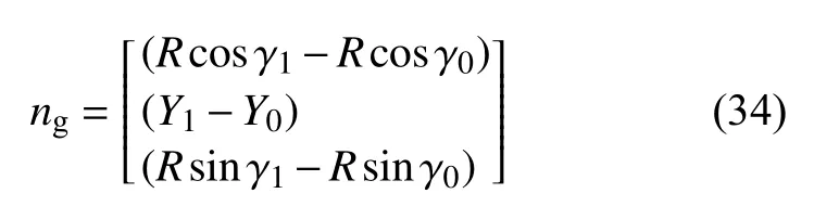
Then, the groove vectorngis:
From Eq. (31) and (34), the following relationship can be used for solution ofng
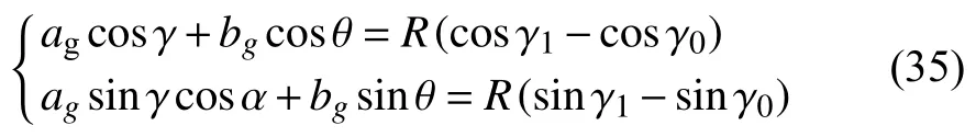
Withγ1andγ0calculated, two unknownsagandbgcan be solved.
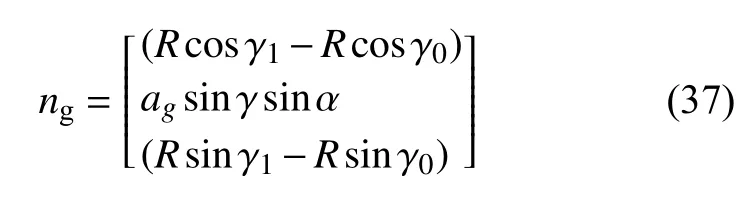
Combining Eq. (31), (34) and (35), theYcomponent of the main groove vector is

The final expression of the groove vectorngis
Hitherto, the solution to the groove vectors of the branch and main pipes have been accomplished, and thus the modeling of the intersecting structure groove. In order to further verify the correctness of the jacket intersecting groove model built in this paper, virtual calculation and simulation is carried out within the MATLAB programming environment.
4 Computational simulation
MATLAB is a commercial mathematical software produced by the American MathWorks Company. It is a highlevel technical computing languages, mainly used for algorithm development, numerical calculation, data visualization and data analysis. It has efficient symbolic calculation and numerical calculation capabilities, thus avoiding a lot of complicated mathematical analysis and operations.Secondly, MATLAB also has a high processing function for graphics operation, which can realize the visualization of programming and calculation results.
4.1 Simulation of intersecting lines
First, the simulation of the intersecting line model is carried out. Assume that the axis intersection angle α=60◦,the main pipe radiusR= 10 cm, the branch pipe radiusr=6 cm, and the eccentric distancee= 1 cm. From Eq. (7), one can know that parametric expressions of the intersection line in theO-XYZcoordinate system can be calculated and simulated in MATLAB, followed by the three-dimensional model of the jacket intersecting structure.
Fig. 4 illustrates the three-dimensional model of the intersecting jacket structure and its corresponding intersecting line. Specifically, Fig. 4 a, b and c are the front view,top view and side view of the 3D model of the intersecting structure, respectively. The horizontal pipe in the figure is the main pipe, and the other is the branch pipe. The angle between the two is 60◦. The red line in the figure is the intersecting line, which is closely attached to the bottom of the intersecting part. Therefore, the intersecting line of the jacket is accurately modelled, as established in the first section of this paper. Fig. 4 d is the intersecting line of the intersecting structure.
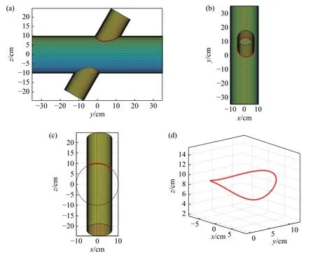
Fig.4 Simulation diagram of the three-dimensional model of intersecting tubes and corresponding intersecting line with α=60° and e=1 cm (a) Front view of the intersecting structure (b) Top view of the intersecting structure (c) Side view of the intersecting structure (d) Intersecting lines
4.2 Simulation of the groove model
On the basis of the intersecting line model established in the previous section, this section uses MATLAB to calculate the dihedral angle, groove angle, and actual cutting angle, and finally solves the groove vectors of two pipes.
Fig. 5 depicts the relationship between the dihedral angle, the groove angle and the position angle of the branch pipe under the axis intersection angle α=60◦. The dihedral angle and the groove angle change continuously with the position angle of the branch pipe. When the branch pipe position angle falls in [0◦,330◦] and [310◦, 360◦] , the dihedral angle φ ≥90◦, and the groove angle ϕ=45◦; when the branch pipe position angle is 330◦to 310◦, the dihedral angle φ<90◦, and the groove angle ϕ=φ/3. The simulation results are consistent with the theoretical relationship between the dihedral angle and the groove angle proposed in Section 2, which indicates the correctness of the above theoretical model.
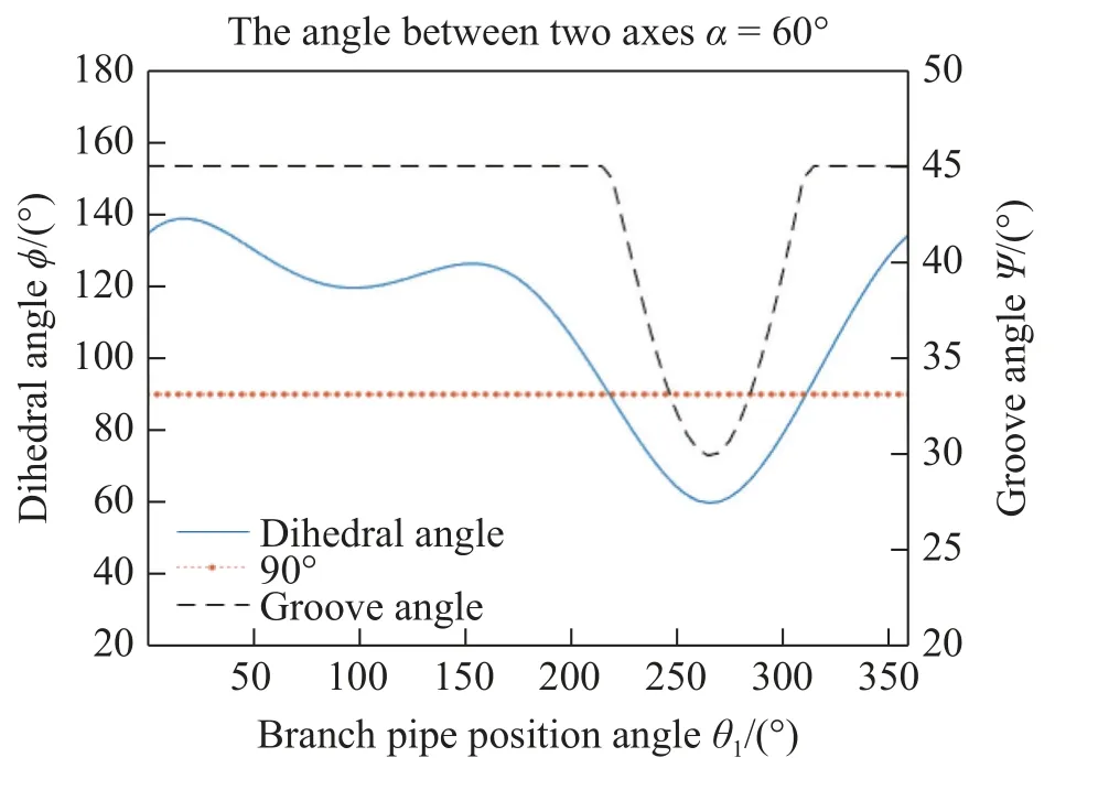
Fig.5 Relationships between the dihedral angle,the groove angle and the position angle of the branch pipe at α =60°
Fig. 6 shows the groove vector of the branch pipe with axis intersection angle α=60◦. From Fig. 6, the groove vector of the branch pipe can be seen more intuitively, as it illustrates the position of the cutting torch on the branch pipe. The green part of the curve in the figure is the intersecting line when the dihedral angle φ <90◦, i.e. the branch position angle from 330◦to 310◦. The curve in the red part is the intersecting line when the dihedral angle φ ≥90◦,where the position angle of the branch pipe is 0 − 330◦and 310 − 360◦. The black arrow outward the intersecting line is the groove vector of the branch pipe. It can be seen that the groove vector of the branch pipe in the red part is different from that in green, because the dihedral angle varies through the intersecting line. It demonstrates that the vector coplanar method proposed in this paper is feasible and correct for solving the branch groove vector.
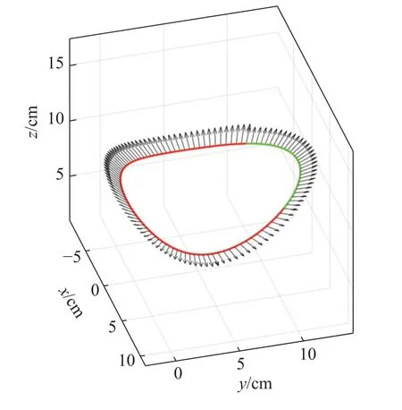
Fig.6 Illustration of the groove vector of the branch pipe at α=60°
In addition, the groove vector of the main pipe can be solved according to Section 3.2. Fig. 7 and Fig. 8 are the side view and top view of the simulated surface of the main pipe groove under the axis intersection angleα= 60°. The curve in the red part in the figure is the corresponding intersecting line for the specific example, and the black line outside the intersecting line is the groove plane made up by the main groove vector. It can be seen that the main groove plane is not a plane, but a curved surface with a certain radius, which confirms the correctness of the above inference,and validates the vector coplanar method proposed in this paper.
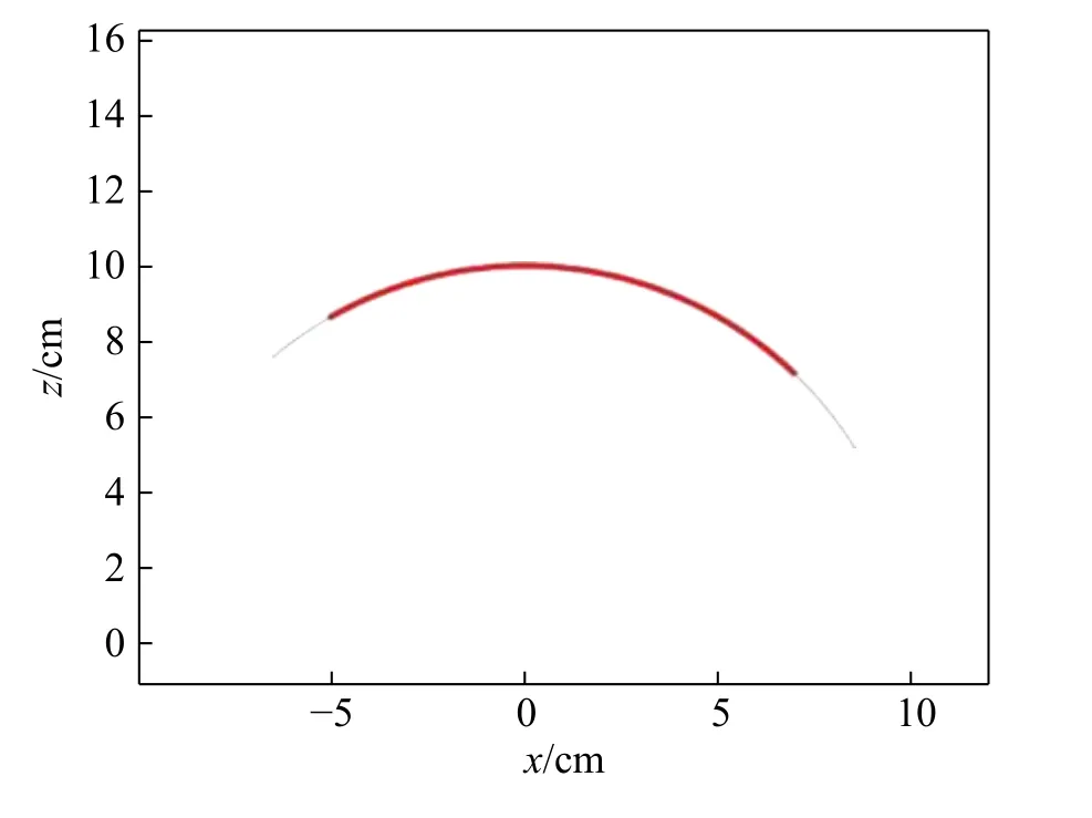
Fig.7 Illustration of the main pipe groove vector at α =60°(side view)

Fig.8 Illustration of the main pipe groove vector at α =60°(top view)
After solving the groove vectors, the groove model of intersecting structures can be digitally illustrated. Fig. 9 simulates a three-dimensional groove under the axis intersection angle α=60◦. The red and green curves in the figure are intersecting lines. The surface composed of black arrows is the branch groove surface on the intersecting line,and the surface around the intersecting line is the main groove surface. The three of them are combined to construct a three-dimensional groove model of the intersecting structure. It can be seen that the shape of the groove changes with the intersecting position. The angle of the groove on the intersecting line does not exceed 45°, which is consistent with the above theory.
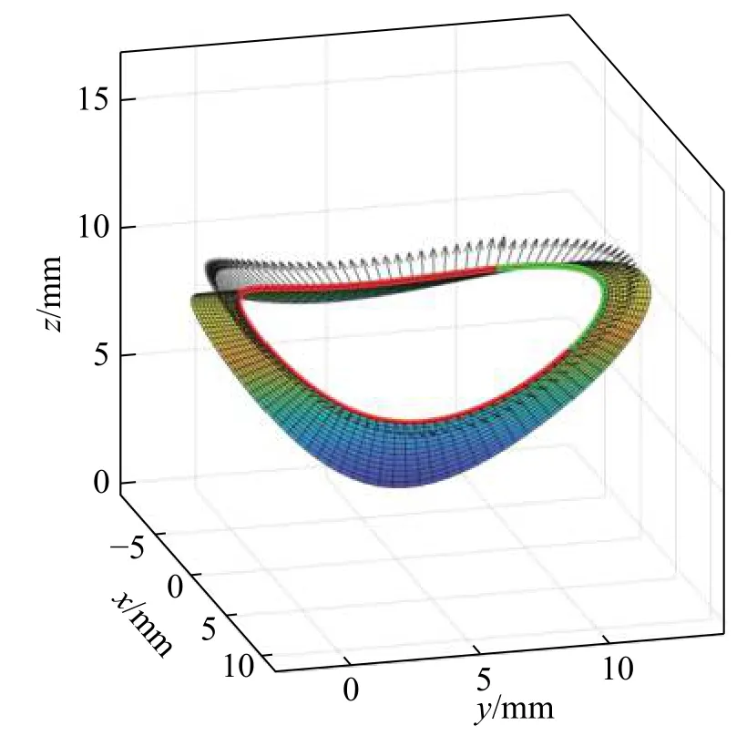
Fig.9 3D simulation of the groove at α =60°
Fig. 10 illustrates the complete simulation of three-dimensional model of the intersecting structure under the axis intersection angle α=60◦. Fig. 11 is an enlarged view of the groove model. Fig. 11 a is an enlarged view of the groove model when the position angle of the branch pipe is from 0 − 330◦and 310° − 360◦. The curved surface of the yellow part in the figure is the branch pipe, and the light green part is the main pipe. It can be found that the main groove is tightly attached to the main pipe, with its shape changing across the intersecting position. The groove angle is equal to 45°. Fig. 11 b is an enlarged view of the groove model with the position angle of the branch pipe from 330◦to 310◦. From the figure, the groove angle is approximately equal to half of the dihedral angle. The simulation results are in good agreement with the relationship between the dihedral angle and the groove angle in Fig. 5. It proves that the vector coplanar method used in this paper to solve the groove vector is correct, and further demonstrates that the groove model of the jacket intersecting structure established in this paper is accurate and feasible.
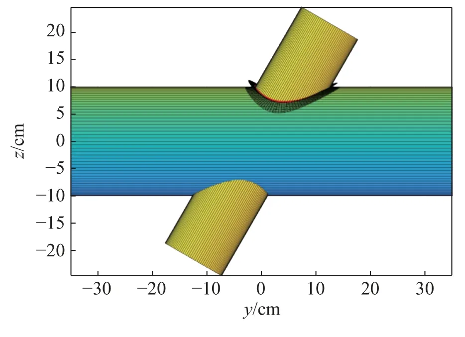
Fig.10 Illustration of intersecting structure at α =60°
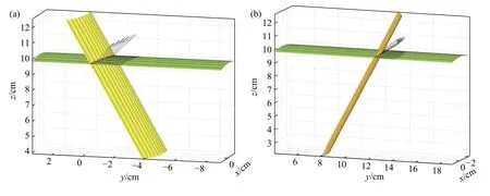
Fig.11 Enlarged view of the groove model of the intersecting structure at α =60° (a) Enlarged view of the groove model when the dihedral angle φ≥90(b) Enlarged view of the groove model when the dihedral angle φ<90
4.3 Creating the graphical user Interface
For convenience, a friendly graphics user interface(GUI) is created in MATLAB. In this paper, the GUI interface is created in the way of FIG (figure), and transformed into an application program independent of MATLAB platform with the editor "MinGW-w64". The designed interface can output required jacket intersecting structure, intersecting line equation, main pipe branch groove vector, 3D model of the groove and the final jacket intersecting groove model after six variable values are input: the radiusRof the main pipe, the radiusrof the branch pipe, the length of the main pipeL, the length of the branch pipe, and the angle α between the two pipes. Fig. 12 illustrates the developed GUI.
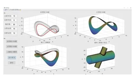
Fig.12 Graphical user interface for the groove model of the intersecting jacket structure
The graphical user interface consists of three modules,namely variable input module, variable output module and graphic display area. The variable input module is the input area for a total of six variables: the main pipe radius, the branch pipe radius, the axis intersection angle, the main pipe, and the length of the branch pipe. The variable output module is the button module. After inputting corresponding parameters, pressing the button will display the corresponding image in the graphic display module.
5 Machined example
To further verify the application potential of proposed method, an intersecting structure was machined by using the CNC intersecting wire cutting machine of KASRY KRXY5. Fig. 13 shows the teaching pendant of KASRY KRXY5 CNC intersecting wire cutting machine. The circular tube has a radius of 50 mm and a length of 400 mm. The branch tube has a radius of 30 mm and a length of 200 mm.The processed branch pipe is orthogonally intersected with the main pipe, and the orthogonal simulation is also carried out in MATLAB.
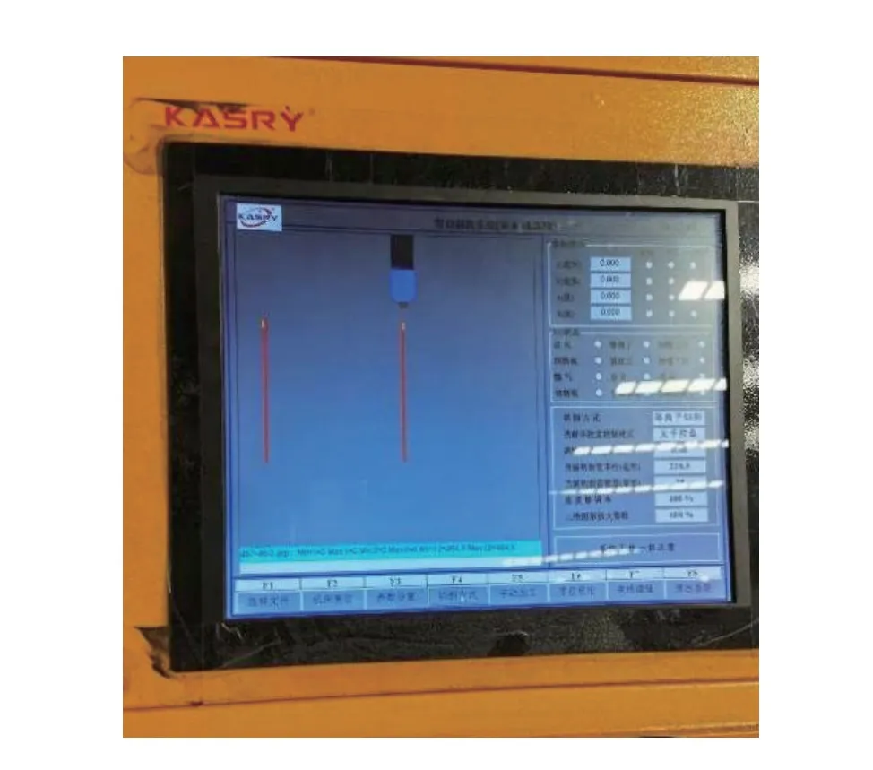
Fig.13 Teach pendant of KASRY KR-XY5 CNC for intersecting line cutting
Fig.s 14 and 15 compare the actual machined structure with simulated orthogonally intersecting pipes. It can be seen from Fig.s 14 and 15 that the machined orthogonal intersecting structure is consistent with its corresponding simulation diagram, which also verifies the correctness of the groove model proposed in this paper.
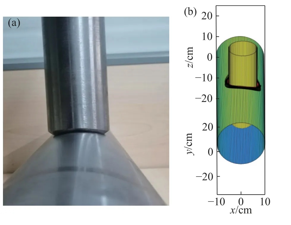
Fig.14 Comparison of machined intersecting structure and MATLAB simulation (main view) (a) The machined orthogonal intersecting structure (b) Orthogonal intersecting structure simulated by MATLAB
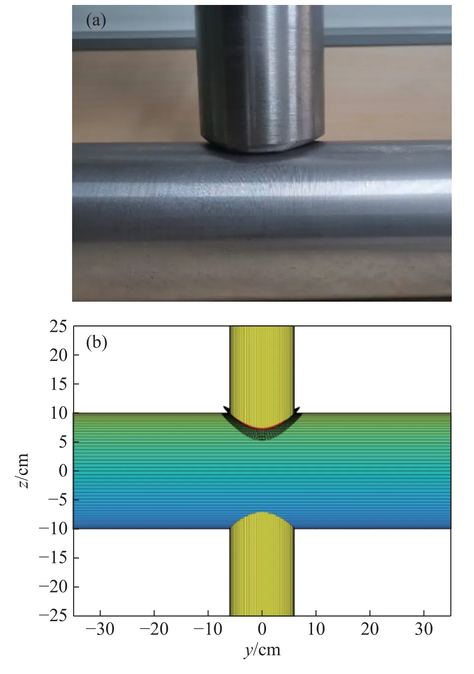
Fig.15 Comparison of machined intersecting structure and MATLAB simulation (Side view) (a) The machined orthogonal intersecting structure (b) Orthogonal intersecting structure simulated by MATLAB
6 Conclusions
(1) The mathematical model of intersecting line is established by spatial analytical method. The proposed new method, i.e. vector coplanar method, can accurately solve groove vectors of intersecting pipes, resulting in establishment of groove model for circular intersecting structures.
(2) Simulation and machining example verification are carried out by MATLAB. The simulation results and machining examples are consistent with the groove model established in this paper, which proves the feasibility and accuracy of the groove model.
- China Welding的其它文章
- The study of arc behavior with different content of copper vapor in GTAW
- Research on stretching flame correction technology of aluminum alloy ship frame skin welding structure
- Application of silver nanoparticles in electrically conductive adhesives with silver micro flakes
- A novel single wire indirect arc metal inert gas welding process operated in streaming mode
- A review of welding residual stress test methods
- Ceramic-copper substrate technology introduction