Review of X-ray pulsar spacecraft autonomous navigation

Yii WANG, Wei ZHENG, Sunnn ZHANG, Minyu GE,Linsen LI, Kun JIANG, Xioqin CHEN, Xin ZHANG,Sijie ZHENG, Fnjun LU

a College of Aerospace Science and Engineering, National University of Defense Technology, Changsha 410073, China

b Key Laboratory of Particle Astrophysics, Institute of High Energy Physics, Chinese Academy of Sciences, Beijing 100049, China

c University of Chinese Academy of Sciences, Chinese Academy of Sciences, Beijing 100049, China

d Beijing Institute of Control Engineering, Beijing 100080, China

e Beijing Institute of Tracking and Communication Technology, Beijing 100091, China

f Aerospace Information Research Institute, Chinese Academy of Science, Beijing 100091, China

g Academy of Military Science, Beijing 100091, China

h National Innovation Institute of Defense Technology, Academy of Military Science, Beijing 100091, China

KEYWORDS

Abstract This article provides a review on X-ray pulsar-based navigation (XNAV).The review starts with the basic concept of XNAV,and briefly introduces the past,present and future projects concerning XNAV.This paper focuses on the advances of the key techniques supporting XNAV,including the navigation pulsar database, the X-ray detection system, and the pulse time of arrival estimation.Moreover,the methods to improve the estimation performance of XNAV are reviewed.Finally, some remarks on the future development of XNAV are provided.

1.Introduction

Advances in the aerospace engineering significantly boost the deep space explorations.The Deep Space Networks (DSNs)can track deep space spacecraft by measuring the ranges and range rates of spacecraft with respect to the ground stations.In this case,the radial positions of spacecraft can be accurately determined, but the components of positions perpendicular to the spacecraft-Earth line have large errors.1Typically,the error of positions perpendicular to the spacecraft-Earth line is around 4 km per Astronomical Unit (AU) of distance between the Earth and spacecraft.2Finally, the uncertainty will grow to a level of the order of ±200 km at the orbit of Pluto and ±500 km at the orbit of Voyager 1.1Therefore, for a deep space spacecraft, it is better to determine the position and velocity autonomously using onboard measurements.The opticalimaging-based autonomous navigation system is welldeveloped, and has been applied to various deep space missions.3However,this method is effective only when a spacecraft is planning to land on a celestial body.4–6Currently,there lacks an autonomous navigation system for a cruising spacecraft.

X-ray pulsar NAVigation (XNAV) system is a promising autonomous navigation system for spacecraft traveling through the solar system.7XNAV employs the X-ray radiation from pulsars to estimate the position and velocity of a spacecraft.A pulsar is a rapidly spinning neutron star, a product of a massive star coming to the end of its lifetime,8and can emit the electromagnetic radiation at regular intervals.The first pulsar was discovered in 1967.9A spacecraft receives electromagnetic signals from pulsars just like a ship receiving signals from a lighthouse on the coast.It is the very reason why pulsars are also called the ‘‘lighthouses in the universe”.10All the pulsars locate far from the solar system,and their positions can be measured in advance.Then,all the pulsars compose an interstellar navigation system.If a spacecraft receives pulsed signals from different pulsars, its position and velocity can be estimated well, just like a vehicle that can autonomously determine its position and velocity by receiving signals from Global Navigation Satellite System (GNSS).It is not a new idea.Voyager 1 and Voyager 2 spacecraft were equipped with the Golden Voyager Record,which marked the position of the Earth with the aid of 14 pulsars.11The Pioneer plaques, fixed to the Pioneer 10 and Pioneer 11, also marked the position of the Earth relative to pulsars.12

This paper will review the development of XNAV.The remainder of this paper is organized as follows.Section 2 introduces the basic concept of XNAV.The missions concerning XNAV are reviewed in Section 3.Section 4 provides the principle of XNAV.Sections 5–7 review the advances of navigation pulsar database, X-ray detection system and pulse Time of Arrival (TOA) estimation, respectively.The methods to improve the estimation peformance of XNAV are briefly reviewed in Section 8.Section 9 concludes the paper and presents the prospects in future work.

2.Basic concepts about XNAV

2.1.Basic concepts of a pulsar

A star in the mass range of about 8 to 30 times the solar mass ends up with a neutron star.The mass of a neutron star is typically 1.4–3.0 solar mass, and the radius of a neutron star is only about 10 km.1Pulsars are rapidly spinning and strongly magnetized neutron stars.

2.1.1.Category

According to the energy source of electromagnetic radiation,pulsars can be classified into three categories1:

(1) Accretion-powered pulsarsAccretion-powered pulsars are within binary systems, which are usually composed of a companion star and a neutron star.The neutron star accretes the matter from the companion star.However,accretion-powered pulsars have a complex spin frequency evolution, and thus are disqualified as reference sources for navigation.13

(2) MagnetarsMagnetars are isolated neutron stars with exceptionally high magnetic dipole fields of up to 1015Gauss.The spin frequency evolution of a magnetar is virtually unstable, which hinders magnetars from being reference sources for navigation.

(3) Rotation-Powered Pulsars (RPP)RPP radiate by consuming the rotation energy of themselves.Most of RPPs can radiate in a broadband (from radio to optical, Xrays and gamma-rays), and are typically recommended for navigation.

According to the spin period, the reciprocal of spin frequency, RPPs can be divided into two types:

(1) Milli-Second Pulsars (MSP)MSPs have spin period less than 20 ms.The period of the fastest pulsar is about 1.4 ms.

(2) Normal pulsarsNormal pulsars have spin periods in the range of tens of milliseconds to several seconds.

2.1.2.Naming convention

The name of a pulsar usually starts with the abbreviation PSR(Pulsating Source of Radio), although pulsars can radiate at other wavelengths of the electromagnetic spectrum meanwhile.PSR is followed by an abbreviation for the epoch,then the pulsar’s right ascension and declination.Pulsars discovered before 1993 use the Besselian epoch.Pulsars discovered after 1993 use the Julian epoch.For example, a pulsar named PSR B1937+21 indicates the pulsar has a right descent of 19h37m and a declination of 21°relative to the Besselian epoch.

2.1.3.Stability of spin frequency of pulsar

Pulsars can be employed to determine the positions of spacecraft, not only because the positions of pulsars can be well determined in advance but also because the spin frequencies of pulsars are quite stable.14The stability of frequency can be scaled by the Square Root Allan Variance (SRAV).When there are N frequency measurements of a source,f1，f2，∙∙∙，fN, the SRAV is defined as15

where ν0is the nominal average frequency of the source.

Ref.15 compares the SRAV of MSPs with the current highprecision timing instruments,including optical clocks,caesium clocks and microwave clocks.It is found that the long-term stability of MSPs is comparable to the current timing instruments.

2.1.4.Pulse profiles of pulsars

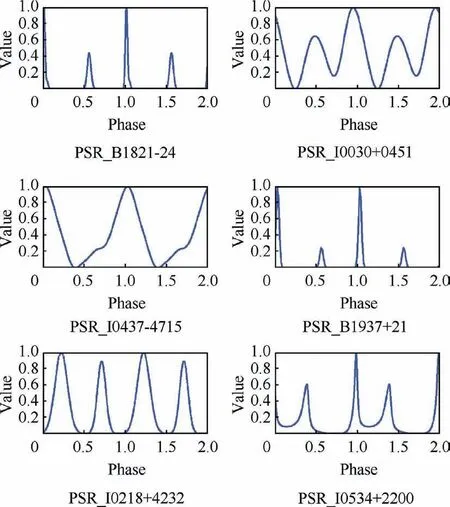
Fig.1 X-ray pulse profiles of pulsars for SEXTANT program.16

The shape of pulsed signals of a pulsar is called profile in the pulsar astronomy community.Each pulsar has a unique profile,just like the fingerprint of a person.Fig.116shows the profiles of pulsars that are selected by the Station Experiment for X-ray Timing and Navigation Technology (SEXTANT) program, which will be introduced in Section 3.2.1.

2.2.Coordinate and time systems for XNAV

In the aerospace engineering, the orbit motion of spacecraft is described in a coordinate system.XNAV employs the coordinate systems identical to other navigation systems, including(A) the J2000.0 Earth-centered inertial coordinate system for Earth-orbiting spacecraft and (B) the J2000.0 heliocentricecliptic coordinate system for deep space spacecraft.17

Given that pulsars locate far away from the solar system,there are numerous huge celestial bodies between pulsars and spacecraft.Given that the space is warped by the gravity of the celestial bodies, the time system for XNAV should take the general relativity effect into consideration.As a consequence,the time system for XNAV is the Barycentric Dynamic Time (TDB) or Barycentric Coordinate Time (TCB).18

3.Past, present and future projects concerning XNAV

Since the first proposal of pulsar navigation and timing,19,20there have been XNAV related projects in the US, China,and Europe.This section will briefly review these projects in chronological order.

3.1.Past projects

3.1.1.USA experiment

The Unconventional Stellar Aspect (USA) experiment is one of the nine experiments on board the Air Force Space Test Program’s Advanced Research and Global Observation Satellite (ARGOS) launched in 1999, and operated from May 1,1999, to November 16, 2000.This experiment consisted of a pair of gas scintillation proportional counters to detect X-ray radiations21(see Fig.2 and a Global Positioning System(GPS) receiver for recording the arrivals of X-ray photons.

The USA experiment diagnosed and corrected a problem with the attitude control of the ARGOS by observing an Xray source,22,23and tried to fulfill the timekeeping using the observation on Crab pulsar.7

3.1.2.XNAV program

The Defense Advanced Research Projects Agency (DARPA)of the United States started a program, X-ray Source Based Navigation for Autonomous Position Determination, which is also referred to as the XNAV program,in 2004.The XNAV program aimed to develop a revolutionary attitude and navigation capability exploiting periodic celestial sources such as pulsars in the X-ray band.24

This program was conceived to last from 2005 to 2010,consisting of three phases.At the end of the program, a flight experiment XNAV was planned to perform on the International Space Station (ISS).However, the whole program was terminated at the end of Phase I (September 2006).Nevertheless, this program performed an in-depth investigation on the feasibility of XNAV, and realized the following achievements24:

(1) Identifying more than 10 candidate pulsars, whose spin stabilities and X-ray fluxes are capable for precise navigation purpose.

(2) Complementation of X-ray detector developments.

(3) Demonstrating navigation algorithms for spacecraft position/velocity determination.

(4) Designing the demonstration system architecture planned for ISS flight.

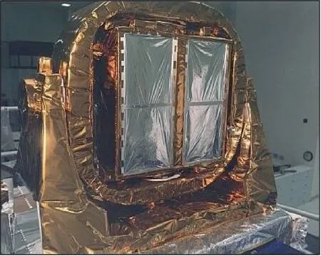
Fig.2 Illustration of USA instrument (image credit: Naval Research Laboratory of the United States).

3.1.3.XTIM program

Between 2009 and 2010,DARPA25performed the X-ray Timing (XTIM) seedling program to study the use of pulsars for time transfer and investigate future demo scenarios.The XTIM was envisioned to create a Pulsar Timescale (PT) by combining long-term pulsar observations with an ultra-stable local clock for short-term stability.The designed XTIM system was expected to have the following potential characteristics25:

(1) Stability: XTIM was based on observations of highly stable pulsars.

(2) Autonomy: XTIM would provide users with an independent and precise measurement of time.

(3) Universality: The pulsars used by XTIM are celestial sources, making them available to any user, anywhere in the solar system.

3.2.Present missions

3.2.1.NICER/SEXTANT program

The Goddard Space Flight Center (GSFC) of the National Aeronautics and Space Administration(NASA)of the US initialized a science mission, Neutron-star Interior Composition Explorer (NICER), in 2011.The fundamental science of NICER is understanding the ultra-dense matter through observations of neutron stars in the soft X-ray band.26Besides the science goal,the NICER mission has a technology demonstration enhancement called Station Experiment for X-ray Timing and Navigation Technology (SEXTANT).16The object of SEXTANT is to perform a real-time, on-board XNAV-only orbit determination with an accuracy of 10 km in the worst-direction, using up to two weeks of dedicated navigation-focused MSP observations.

The SEXTANT is the first real-time flight experiment on XNAV in the world.As shown in Fig.3,16the system architecture of SEXTANT includes four main components: (A) the NICER X-ray Timing Instrument (XTI), (B) the flight software and algorithms, (C) the ground system, and (D) the ground testbed.27In 2018,SEXTANT has successfully demonstrated the XNAV aboard the ISS and achieved a positioning error below 10 km.28

Fig.3 SEXTANT system architecture.16

3.2.2.PULCHRON project

In December 2018, the European Space Agency (ESA)announced a project called PULCHRON, an abbreviation built with the words ‘‘Pulsar” and ‘‘Chronos”, the ancient Greek term for‘‘Time”.29The primary object of PULCHRON is to demonstrate the effectiveness of a pulsar time scale for the generation and monitoring of system timing in Positioning,Navigation and Timing (PNT) in general, and of Galileo System Time (GST) in particular.

The PULCHRON project is composed of (A) Pulsar Measurement Collection System (PMCS), (B) Pulsar Frequency Standard Unit (PFSU) and (C) Pulsar-Augmented Clock Ensemble(PACE),30where PMCS monthly collects the pulsar measurements from the European Pulsar Timing Array(EPTA), which includes Effelsberg, Lovell, Westerbork, Nanc¸ay and Sardinia31; PFSU aims to realize the physical pulsar time scale; and PACE builds a posteriori ‘‘paper” time scale mixing pulsar data and GNSS station and satellite clocks.

3.2.3.XPNAV-1 satellite

China launched an experiment satellite called X-ray Pulsar navigation-1 (XPNAV-1) in November 2016.The objective of XNAV-1 is to test the technology of pulsar observation in the soft X-ray band with the X-ray instruments developed by China Academy of Space Technology (CAST).32

Up to now, the XPNAV-1 has accomplished observations on 4 isolated RPPs and 4 X-ray binaries,32performed a rough orbit determination with an averaged accuracy about 38.4 km,33and completed a timely observation on the glitch of Crab pulsar.34

3.2.4.Navigation study of POLAR

POLAR was a hard X-ray polarimeter aboard the Chinese space laboratory TianGong-2 (TG-2), which was launched in 2016 and deliberately de-orbited in July 2019.It was equipped with an array of 1600 plastic scintillators for precisely and efficiently measuring the linear polarization of hard X-rays.During the mission, POLAR detected 55 γ-ray bursts.

Besides observing the γ-ray bursts, POLAR performed a navigation study.The orbit of TG-2 was determined to have an accuracy of about 10 km with 31-day-long hard X-ray data on Crab pulsar.The feasibility of XNAV was validated in principle.35

3.2.5.Navigation study of Insight-HXMT

The Insight-Hard X-ray Modulation Telescope (Insight-HXMT),China’s first X-ray astronomy satellite,was launched in June 2017.The main scientific objectives of Insight-HXMT include: (A) scanning the Galactic Plane to find new transient sources and to monitor the known variable sources, (B)observing X-ray binaries to study the dynamics and emission mechanism in strong gravitational or magnetic fields, and(C) monitoring and studying Gamma-Ray Bursts (GRBs)and Gravitational Wave Electromagnetic counterparts(GWEM).36

Besides accomplishing the scientific objects,Insight-HXMT completed a flight study on XNAV by employing the X-ray data of the Crab pulsar collected between August 30 and September 3, 2017.As a result, it was claimed that Insight-HXMT can locate itself with an error below 10 km (3σ).37,38

3.3.Future missions

3.3.1.CubeX

The SEXTANT team is working with scientists from Smithsonian Astrophysical Observatory and Harvard University to test XNAV on a CubeSat mission called CubeX.CubeX plans to employ an X-ray telescope to identify and spatially map lunar crust and mantle materials excavated by impact craters,and also serves as a pathfinder for autonomous precision deep space navigation using X-ray pulsars.39

3.3.2.XNavSat

The Indian Institute of Space Science and Technology is developing a small satellite mission called XNavSat.This mission aims to calculate the true anomaly of the satellite in real time,assuming that the remaining orbital elements of the satellite are known.40

4.Principle of XNAV

4.1.XNAV for a single spacecraft

The basic idea of XNAV for a single spacecraft is similar to that of GNSS.When a spacecraft receives signals from a pulsar, the TOAs of the signals, tSC, can be measured.

Given that the spin frequency of pulsar is stable,the evolution of the pulse phase of pulsar at the Solar System Barycenter (SSB) can be described by

where F0，F1and F2are the spin frequency of the pulsar at T0,its time derivative and its second order time derivative respectively.φT0is the phase at T0.In practice, F0，F1and F2can be found in the public pulsar ephemerides.41,42

Eq.(2) is essentially a Taylor expansion of the pulse phase around the pulse phase at T0.If the high orders of the time derivatives of the spin frequency of a pulsar are taken into consideration,the pulse phase evolution should be described more accurately than Eq.(2).However, in practice, the spin frequency and its time derivative families are fitted by the real pulsar data.Up to now, the observation on pulsar has lasted for 55 years,43and the current pulsar ephemerides only contain the second-order time derivative of spin frequency at most.

In Eq.(2), tSSBis expressed as44

where rSSB（t ） is the position of the spacecraft relative to the SSB,n denotes the direction vector of the pulsar,G is the gravitational coefficient, Mkis the mass of the kth celestial body,rk（t ） is its position relative to the spacecraft, c is the speed of light, and ‖• ‖ denotes the ℓ2-norm of the vector within.

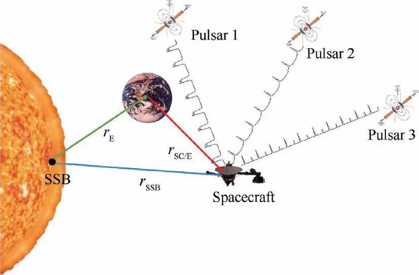
Fig.4 Principle of XNAV for a single spacecraft.

It can be learned from Eq.(3) that rSSB（t ） projected on the direction of pulsar, nTrSSB（t ）, can be obtained if tSSBand t are available.When the spacecraft receives signals from three pulsars simultaneously(see Fig.4),rSSB（t ）can be determined via a nonlinear least squares method just like the way to determine the position via GNSS.45If there are not three pulsars available at the same time,the position of the spacecraft can be estimated by combining the orbit dynamics information with pulsar signals.46

4.2.XNAV for multi-spacecraft

Fig.5 shows two spacecraft observing one pulsar.Assumeandare the pulse TOAs at spacecraft A and spacecraft B,respectively.According to Eq.(3), we have

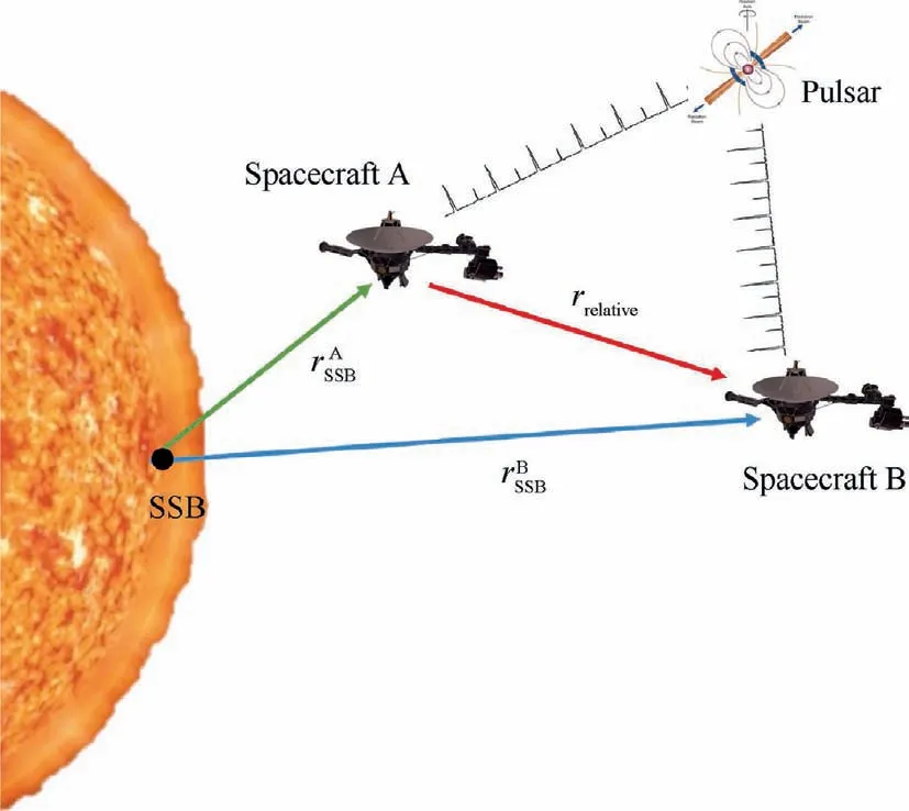
Fig.5 Principle of XNAV for multi-spacecraft.

Table 1 X-ray navigation pulsars selected by past and present missions.

4.3.Techniques supporting XNAV

As shown in Eqs.(2), (3) and (5), the techniques supporting XNAV are:

(1) Navigation pulsar database: Pulsars for XNAV are like navigation satellites for GNSS.Unlike the man-made satellites,the location,brightness and modulation properties of pulsars cannot be designed.Thus,pulsars qualified for navigation are rare and their ephemerides need to be updated timely.

(2) X-ray detection system: X-ray detection system for XNAV are like GNSS receivers for GNSS.They detect and record X-ray photons from pulsars.

(3) Pulse TOA estimation: Pulse TOA is an important and basic parameter for XNAV, as illustrated in Eqs.(3)and (5).However, a spacecraft can only record a series of photons instead of a continuous pulsed signal given that the flux of a pulsar is extremely weak.Moreover,the spacecraft keeps performing an orbit motion, which causes the extraction of pulse TOA from the recorded photons more complex.As a consequence, it is a great challenge to get a reliable and precise pulse TOA.

The advances of the above three techniques will be sequentially introduced in Sections 5–7.

5.Navigation pulsar database

As illustrated in Section 2.1.1,RPPs are recommended for navigation.Currently, 2200 RPPs have been discovered,49among which about 150 pulsars emit X-ray radiation.50Approximately 10% pulsars are MSPs.1MSPs are the most promising reference sources for XNAV because they exhibit very high timing stabilities, which are comparable to the current atomic clocks.51,52

The Crab pulsar(or PSR B0531+21)is selected by all missions.Although the Crab pulsar is not a MSP and has glitches in which the spin parameters change suddenly,53it is much brighter in X-ray than the other pulsars.Therefore, the Crab pulsar can be easily detected and can provide a much more accurate pulse TOA than MSPs when the Crab pulsar and MSPs are observed for the same duration.

The navigation pulsar database contains the following information that describes the timing and location properties of the selected pulsars:

(1) Position parameters including the declination, the right ascension, and the proper motion of pulsar;

(2) Frequency evolution parameters including the spin frequency and its first- and second-order time derivatives;

(3) The other necessary parameters including the absolute pulse phase for a given epoch, the version of planet ephemerides (NASA’s Jet Propulsion Laboratory(JPL) ephemerides for example), the orbit parameters of binary pulsars, etc.

In practice, the navigation pulsar database is supported by the pulsar timing analysis,which is usually performed by global pulsar timing programs.For example, the North American Nanohertz Observatory for Gravitational Waves (NANOGrav) project54has been timing several pulsars in the pulsar database of SEXTANT program,55the Jodrell Bank observes the Crab pulsar,42and the Parkes Pulsar Timing Array(PPTA)monitors 20 pulsars.56Table 123,33,37,55,57shows the navigation X-ray pulsars used by the past and present missions.

6.X-ray detection system

The pulse X-ray emission of a RPP is usually non-thermal,which has a power law spectrum with a photon index of about-2, i.e., the flux of the pulse photon in the soft X-ray band(photon energy less than 10 kilo electron Volt (keV)) is much higher than that in the hard X-ray band (energy above 10 keV).57,58More photons indicate a more accurate pulse TOA estimation(see Section 7).Therefore,the soft X-ray radiation from pulsars is recommended for navigation.The background, which comes from the diffuse Cosmic X-ray Background (CXB), space particles and the non-pulse portion of the pulsar, is commonly detected along with the X-rays of pulsars.58As a consequence, an X-ray detection system consists of an optics system, designed to focus X-ray photons,and an X-ray detector counting X-ray photons collected by the optics system.

6.1.Optics system

Two broad categories of optics systems are used in XNAV observations:collimators and focusing X-ray telescopes.A collimator restricts the Field of View (FOV) of the whole detection system.In this way,only the background within a narrow portion of the space can enter the detection system.On the other hand, a focusing X-ray telescope focuses the source flux onto the X-ray detector in the focal plane.59As will be seen in Section 6.1.2,only the background arriving within a small incidence angle can be collected.Therefore, both the collimator and focusing X-ray telescope can effectively reduce the background.

6.1.1.Collimators

Fig.659shows a simple slat collimator with an FOV of arctan （a/h）×arctan （b/h ） where a，b and h are the length,width, and height of a slat respectively.All photons or particles arriving at angles larger than arctan （a/h） and arctan （b/h） are attenuated by the walls of collimator structure.In other words,the photons or particles from the sources with angular positions relative to the targeted source outside the FOV are rejected.Thus,for collimators,a small FOV indicates a strong capability of rejecting background.

Because of their simple structures,collimators were used in a number of X-ray missions including Uhuru, the first X-ray satellite launched in 197060(see Table 236,60–68).Collimators are also used in X-ray imaging, with scanning observations and image reconstruction techniques.69

6.1.2.Focusing X-ray telescopes

X-rays can be focused with the grazing incidence optics.The mirrors comprising focusing X-ray telescopes are typically multi-shell like structures coated with a heavy metal, such as gold or nickel.70Soft X-ray photons can be reflected from the surface of mirror, when their angles of incidence with respect to the surface are less than71

where ρ is the density of coating material and E is the energy of photon.

The reflectivity of gold is a function of energy and angle of incidence,71which increases as the energy and angle of incidence reduce.In practice,the angle of incidence is typically less than 1°.However, a low angle of incidence can be achieved at the cost of a long focal length of the telescope.

In order to achieve a good reflectivity and good imaging quality, focusing X-ray telescopes require much precise figuring and ultra-high-quality mirrors with roughness better than 1 nm.59The above requirements all indicate that the fabrication of focusing X-ray telescopes is expensive and laborintensive.

Fig.6 A simple slat collimator.59

For a focusing X-ray telescope,its effective area depends on the energies of incoming photons because the reflectivity is a function of photons’ energies and thus is with the unit of‘‘cm2@b keV”, where @bkeV means ‘‘at b keV”.Besides this,the angular resolution quantified by the Half-Power Diameter(HPD)is also an important parameter to describe the imaging capability of a focusing telescope.72HPD is defined as the angular diameter in the focal plane, which contains half the flux (at a given energy) focused by the telescope.

Although there are various geometries that can achieve grazing incidence optics,73the Wolter-I geometry is most frequently used in X-ray telescopes (see Table 370,72,74–91).Since the FOV of a Wolter-I geometry is small, recently, a lobstereye geometry is used to achieve wide field X-ray imaging.A lobster-eye geometry can observe simultaneously multiple sources locating relative far away,such as 10°from each other,and can monitor transient X-ray sources.This section will focus on the two geometries.

(1) Wolter-I geometry

Almost the focusing X-ray telescopes that have been in orbit were fabricated in accordance with or approximating the Wolter-I geometry80with the principle shown in Fig.7.92The incoming rays experience two grazing incidence reflections from two confocal paraboloidal and hyperboloidal mirrors sections.Several pairs of paraboloidal and hyperboloidal mirrors can be nested to increase the effective area.Fig.8 shows the nested mirrors on the Chandra X-ray Observatory.

(2) Lobster-eye optics

This optics mimics the eyes of lobsters and was suggested independently by Schmidt93in 1975 and by Angel94in 1979.The Schmidt arrangement employs the orthogonal sets of mirrors (see Fig.9) and and the Angel arrangement utilizes array of reflecting cells (see Fig.10).The lobster-eye optics has a wide FOV, up to maximum of 2π.95This feature makes the lobster-eye optics more suitable for the all-sky survey than the Wolter-I geometry,the FOV of which is typically less than 1°.96,97

The lobster-eye optics can be constructed as a one-Dimensional (1D) or two-Dimensional (2D) system.The Schmidt arrangement shown in Fig.9 is a 2D system, which consists of two orthogonal 1D systems.The Angel arrangement is also a 2D system.The incoming photons focused to form a point with tails forming a cross like image, in which the photons at the center point are reflected twice and those in the wings are only reflected once.98It appears that the Schmidt arrangement can practically achieve an angular resolution of the order of one tenth of a degree or better, and the angular resolution of the Angel arrangement can be as good as a few arc seconds, if very precise reflecting cells can be fabricated.95

Nowadays, both the Schmidt and Angel arrangements are under development.Ref.95 designs an X-ray optics system for CubSat demonstrator based on the Schimdt arrangement.Ref.99 uses the microchannel plate technology to fabricate the reflecting cells in the Angel arrangement.Ref.100 employs the micro-pore optics to realize the Angel arrangement.

In the near future, the Einstein Probe (EP)101will employ the lobster-eye optics to form a large FOV monitor to detect X-ray transients and gamma-ray bursts.In order to test the lobster-eye optics for EP, the EP-WXT Pathfinder, an experi-mental module for the Wide-field X-ray Telescope (WXT) of EP, was loaded on the satellite SATech-01 launched on July 27, 2022.The EP-WXT Pathfinder released on its first results on August 27,2022.The Space-based multi-band astronomical Variable Objects Monitor (SVOM)102,103will employ a narrow-field-optimised lobster-eye telescope to promptly detect and accurately locate gamma-ray bursts afterglows.These two satellites will be launched in the next couple of years.

Table 2 Past and active X-ray telescopes employing collimators.

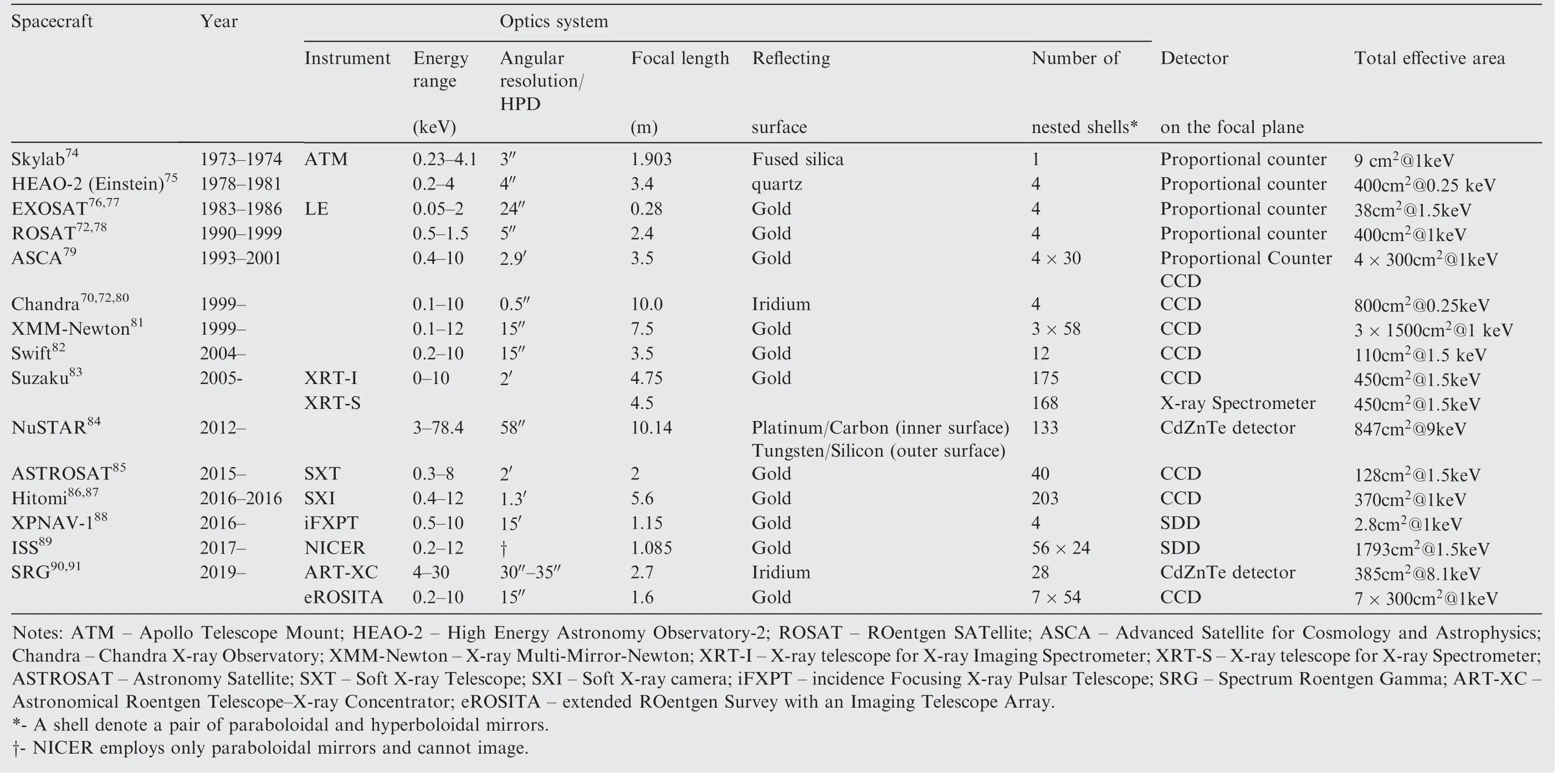
Table 3 Past and active X-ray telescopes using Wolter-I geometry.

Fig.7 Principle of Wolter-I geometry.92

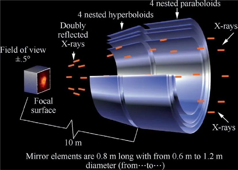
Fig.8 Nested X-ray mirrors on Chandra X-ray Observatory(Image credit: NASA, Chandra, and the Smithsonian Astrophysical Observatory.).

Fig.9 Schmidt arrangement for a lobster-eye geometry.

6.2.Detectors

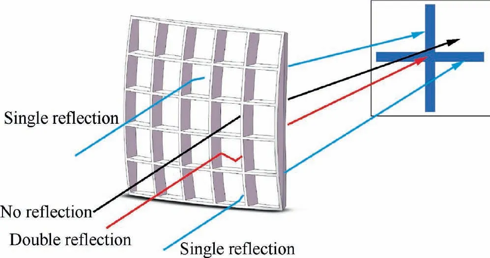
Fig.10 Angel arrangement for a lobster-eye geometry.

X-ray detectors aim to turn the collected X-rays into electronic signals and further into data that can be stored for later analysis.104These data typically include the arrival time, energy,and the location on the detector of each photon detected.The commonly used X-ray detectors are proportional counters,Charge-Coupled Devices(CCDs),Silicon Drift Detectors(SDDs), scintillation detectors, CdZnTe detectors, etc.

6.2.1.Proportional counters

Proportional counters were stemmed from gases detectors,which were first applied to detect cosmic rays and other particles in laboratory,105and have been used in soft X-ray astronomy for nearly six decades.

A standard proportional counter is a gas-filled chamber with a coaxial thin wire as shown in Fig.11.The electrical field is generated by applying positive High Voltage (HV) to the anode.106X-rays entering the chamber ionize the gas, producing electrons.The electrons can be accelerated in the electric field and further ionize gas atoms by collisions and cause charge multiplication.In proportional counter, the HV is tuned to maintain a linear relation between the input photon energy and the charge.104This is the very reason for its name.

As shown in Tables 2 and 3, the combinations of proportional counters and collimators were widely applied to X-ray astronomy satellites, especially those launched before 2000.It is because, the observation of the weak photon fluxes from cosmic X-ray sources with non-imaging detection systems(detectors with collimators) requires large-area detectors, which can be realized by multi-anode multilayer proportional counters under the level of fabrication then.

In order to improve the energy resolution of the proportional counter, the Gas Scintillation Proportional Counter(GSPC) was proposed107and used aboard the EXOSAT.108However, GSPCs have now been superseded by CCDs (see Section 6.2.2) for soft X-ray band and CdZnTe detectors (see Section 6.2.5) for hard X-ray band.104

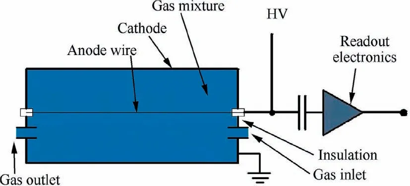
Fig.11 Schematic diagram of a proportional counter.

Proportional counters may suffer from an aging problem because of the cracking of gas molecules during normal operation.109The USA experiment (see Section 3.1.1) was aborted because of the leakage of gases filled in the proportional counters.

6.2.2.CCD

The CCD was invented at Bell Laboratories in 1969, and was first employed as the focal plane detector for X-ray imaging by the ASCA satellite in 1993.Since then, CCDs are the most widely used detectors in X-ray astronomy because a CCD detector usually has small pixel size, large chip size, good energy resolution, and low noise.110

A conventional CCD is an array of small and thin electrodes of metal–oxide–semiconductor capacitors.The incoming X-rays interact with the semiconductor substrate,producing electron–hole pairs.An electric field can be produced,when the gates between neighboring pixels have potentials.110In this way, the electrons can be stored in pixels, and can be transferred, pixel to pixel, from the semiconductor to a readout amplifier, by tuning the gate potentials (see Fig.12111).

Although CCDs have a high energy resolution up to about 130 eV@6 keV and a spatial resolution on the order of 10 μm,their read-out typically cost several seconds.112In order to accelerate the read-out, two variations on CCD have been designed, including the pnCCD113and the Swept Charge Devices (SCD).114In a pnCCD, the pixels are aligned as column parallel, and each column has a dedicated readout channel.115,116In an SCD, the electrons generated by interactions between X-rays and the semiconductor substrate are simultaneously or consecutively swept towards the central diagonal channel, and then are transferred to the single read-out node located in one corner of the devices (see Fig.13).In this way, an SCD can improve the time resolution at the cost of sacrificing imaging capability.117Up to now,pnCCD has been applied to the XMM-Newton and eROSITA,and will operate on the SVOM and EP.SCDs have been applied to the Insight-HXMT.

6.2.3.SDD

Fig.12 Electrons transfer principle for a 3×3 pixels CCD.111

Fig.13 Schematic diagram of SCD.

SDDs were first proposed in 1983.118An SDD consists of a radial electric field,which terminates in a very small collecting anode on one face of the device (see Fig.14).Electrons generated by the interactions between X-rays and the semiconductor are guided along these electric field lines to the anode.On the other hand, a small anode indicates a low device capacitance,and finally produces a small electronic noise.119Electrons move fast in the electric field,and so can be collected in a very short time.SDDs thus have a very high time resolution.However,one SDD pixel needs one read-out channel,which makes it almost impossible to obtain high spatial resolution images like CCDs.

SDDs have been successfully applied to NICER and XNAV-1, and are planned to be employed by CubeX, XNav-Sat and the enhanced X-ray Timing and Polarimetry(eXTP).120

6.2.4.Scintillation detector

Scintillation detectors are employed to detect X-rays with energies higher than several keV.A scintillation detector is a combination of a crystal, which emits optical light photons when absorbing X-ray photons, and a light sensor, which collects the optical photons110(see Fig.15).The light sensors are typically Photo-Multiplier Tubes (PMT), photodiodes, silicon photo-multipliers,and SDD.In practice,a phoswich,a combination of two different crystals,is usually employed instead of a single crystal.The NaI(Tl)/CsI(Na) phoswich has been applied to RXTE121and Insight-HXMT.122

6.2.5.CdZnTe detector

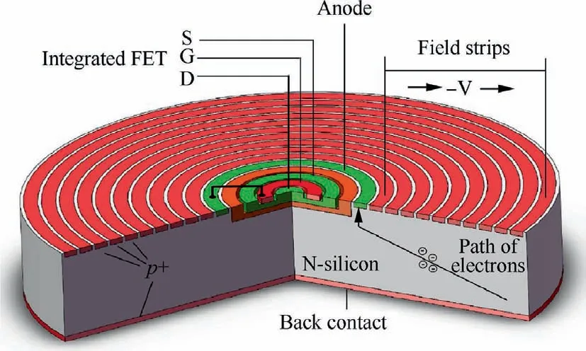
Fig.14 Schematic diagram of SDD.

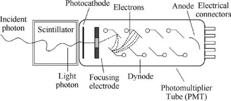
Fig.15 Schematic diagram of a scintillation detector comprising a scintillation material coupled to a PMT.

Cadmium Telluride (CdTe) and Cadmium Zinc Telluride.(CdZnTe) detectors are semiconductor detectors with a function principle similar to SDDs.However,in CdZnTe detectors,the electrons collected in each pixel are read out independently.104Nowadays, CdZnTe detectors become the modern standard instrument for detecting X-rays with energies above several keV, and have been applied to Swift and NuSTAR.

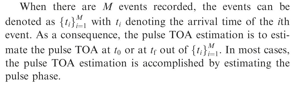
7.Pulse TOA estimation

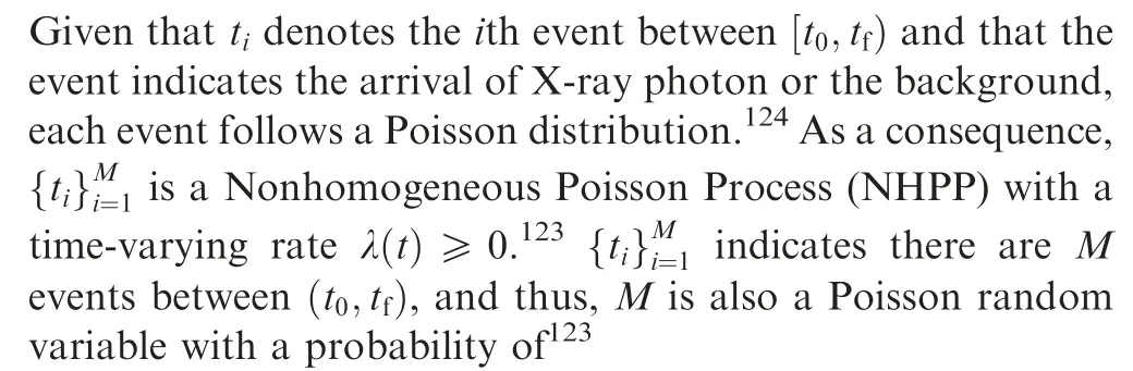
Given the large distance and so the low X-ray flux of a pulsar,a pulsar cannot be detected to have regularly distributed pulses like a beacon.In this case,a spacecraft can only record a series of events within an exposure, which lasts from t0to tf, on a pulsar.123It should be noted that an event indicates not only the arrival of an X-ray photon from the pulsar but also possibly the arrival of the background, which could come from CXB, space particles and the nebula surrounding the pulsar.

7.1.Pulsar signal model

λ（t ） can be expressed as

where h（φ ） is the periodic pulse profile or template, φdet（t ） is the detected phase, α and β are the known pulsed count rate and background count rate,respectively,and counts/s denotes‘‘counts per second”.

Assuming the spacecraft is performing a linear uniform motion towards the pulsar or being stationary, φdet（t ） in Eq.(8) is expressed as

where φ0is the pulse phase at t0and f0is the frequency of the detected pulsar signal.If the spacecraft is stationary, f0=F0.When the spacecraft moves towards the pulsar along a line,f0becomes

where v is the velocity of spacecraft along the spacecraft-pulsar line.

Taking the SEXTANT program as an example, Fig.1 shows the pulse profiles of six pulsars, and Table 455provides α and β of the pulsars selected by the program.As shown in Table 4,55the background count rates of all pulsars are at least one order of magnitude higher than the pulsed count rates.Although the Crab pulsar has the highest pulsed count rate among the pulsars,its background count rate is still two orders of magnitude higher than its pulsed count rate.It indicates that all the X-ray pulsars are very faint sources.Moreover,the arrival of photons or background is random, which indicates that the pulse phase estimation belongs to the stochastic signal processing.

7.2.Basic pulse phase estimation frames

The basic pulse phase estimation problem is to estimate φ0in Eq.(9)under the assumption that the spacecraft is performing a uniform linear motion toward the pulsar or stationary and that the evolution of spin frequency of pulsar is ignored.

This section introduces the current methods to solve the above problem.These methods can be divided into two classes:(A) estimating φ0using epoch folding, and (B) estimating φ0with the direct use of

7.2.1.Pulse phase estimation using epoch folding

(1) Estimation with known f0.

When f0in Eq.(9) is already known, the period of pulsar signal equals to P=1/f0and an empirical profile can be recovered from.This recovery method is called epoch folding.

Assuming the exposure [t0，tfcontains N periods,the epoch folding consists of three steps: (A) dividing the ith(i=1，2，∙∙∙，N) period into Nbbins, each lasting for Tb=P/Nb; (B) the events falling in the jth bin of the latter periods are folded back into the jth bin of the first period(see Fig.16); (C) the event counts in each bin are normalized.Finally, an empirical profile is recovered.The statistical properties of the empirical profile have been investigated in Ref.123.It should be noted that the epoch folding is applied not only to XNAV but also to X-ray pulsar astronomy.125,126This paper focuses on the application of epoch folding on XNAV.

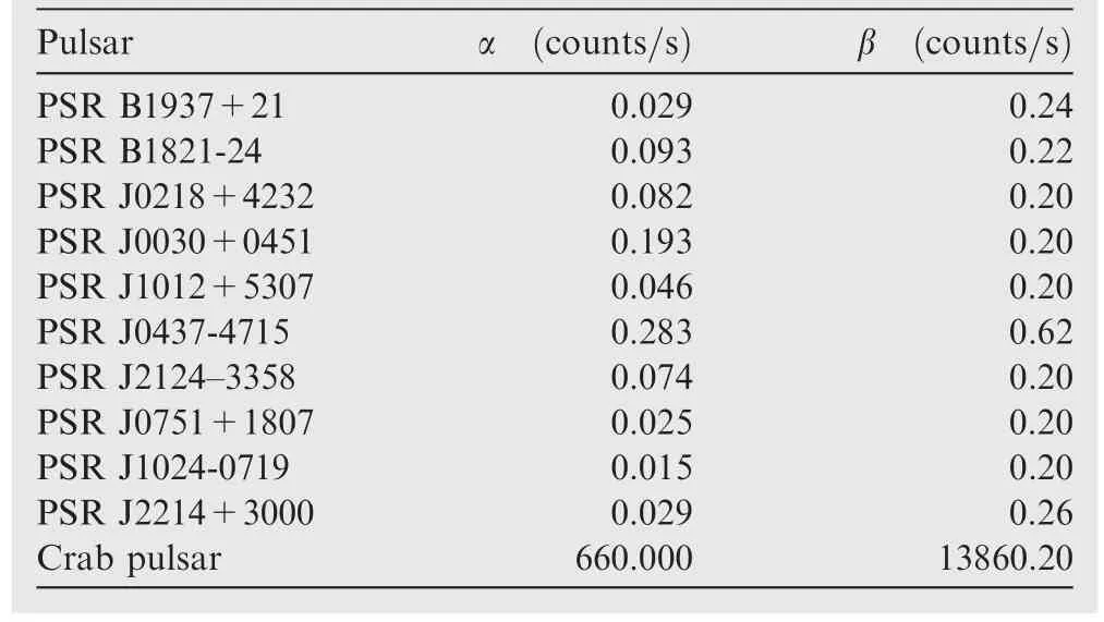
Table 4 Pulsed count rates (α) and background count rates(β) of pulsars selected by SEXTANT program.55

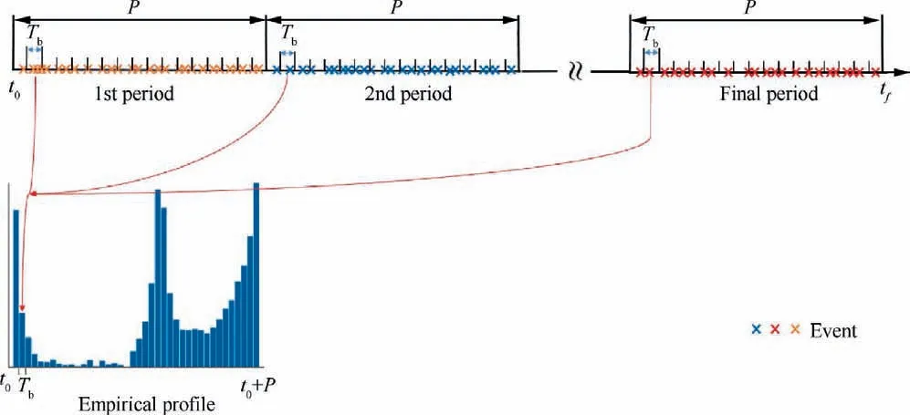
Fig.16 Epoch folding procedure of a pulsar.

The phase offset between the recovered empirical profile and the template is called φ0.Thus, the estimation of φ0can be recast as the classical problem of estimating phase delay between two waveforms.The classical methods to estimate φ0are cross-correlation47and Nonlinear Least Square(NLS).123The Cramer-Rao Low Bounds (CRLBs) for the φ0s estimated by cross-correlation and NLS are derived in Refs.123,47.

Motivated by Refs.123,47, many works started to pursue the fast computation, which is typically accomplished by Fast Fourier Transformation (FFT).For an empirical profile with Nbbins, the computational complexity of cross-relation127with the aid of FFT is about O NblogNb, much less than NLS (about O).FFT is also utilized by Refs.128,129,the bispectrum with the aid of FFT is applied in Ref.130,and the Discrete Fourier Transformation (DFT) is employed by Ref.131.

(2) Estimation with unknown f0.

When f0in Eq.(9) is unknown, we should first estimate f0and then estimate φ0with the methods discussed above.

The estimation of f0is commonly solved by finding the period of a pulsar.Table 5132–144lists the current period finding algorithms, in which the Lomb–Scargle, Generalized Lomb–Scargle and Correntropy kernel periodogram find the period in the frequency domain, and the other algorithms belong to time-domain methods.Although those methods are derived from different principles, they are dependent on the qualityof the light curve of the pulsar.When the exposure on the pulsar is short and the pulsar has a faint magnitude,the quality of the final light curve is low and all those methods become inefficient.145

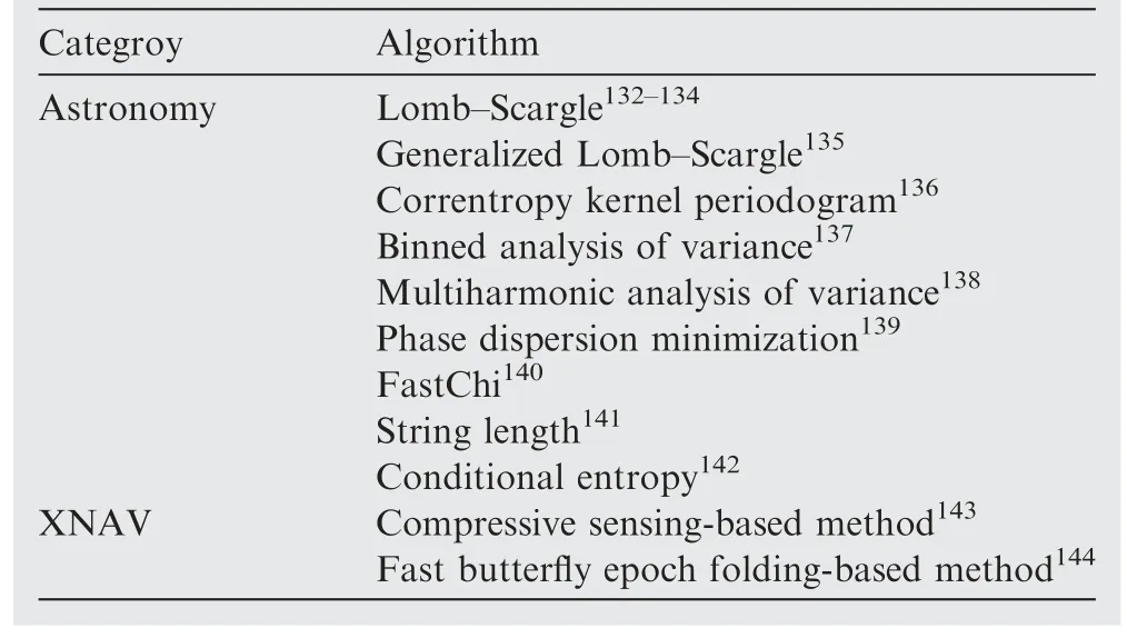
Table 5 Current period finding algorithms.

7.2.2.Pulse phase estimation with direct use of events

When f0in Eq.(9)is known,according to Eqs.(7)–(9),the Mdimensional joint probability density ofis123

Eq.(11) can be recognized as the likelihood function, and the Log-Likelihood Function (LLF) is

The Maximum Likelihood Estimator(MLE)is provided by maximizing Eq.(12)with respect to the unknown φ0.The second term on the right side of Eq.(12)is not sensitive to φ0.As a consequence, the estimate of φ0，^φ0, can be expressed as

where arg max （• ） denotes the argument of the maximum of the function within （• ）.

If f0in Eq.(9)is unknown,the right side of Eq.(12)can be viewed as a function of φ0and f0.Then, φ0and f0can be estimated simultaneously by maximizing Eq.(12).In this case,we have

As shown in Eq.(14), MLE provides a more flexible frame to estimate φ0and f0than the epoch folding method.In other words, if the evolution of spin frequency is taken into consideration,MLE can also work well,and can provide a result closer to the CRLB than NLS.123

Eq.(14)is usually solved by a two-dimensional grid search.When the grid for search is Nφ×Nf, the computational complexity of the MLE is about O Nφ×Nf×M , which is much higher than the computational complexity of NLS even when Nb=Nφ=Nf.In order to accelerate the computation of Eq.(14),the intelligent optimization method is employed.146However,the intelligent optimization method that utilizes the technique of random numbers cannot have a stable estimation result.146

7.3.On-orbit pulse phase estimation

The methods introduced in Section 7.2 are based on the assumptions that the spacecraft is stationary or performs a linear uniform motion towards the pulsar.However, in practice,spacecraft orbit around a central celestial body, such as the Earth for the Earth-orbiting satellites or the Sun for deep space spacecraft.147In this case, f0in Eq.(9) is time-varying and unknown, and then, Eq.(9) can be rewritten as148

where

where fsis the spin frequency of the pulsar and θd（t ） is the phase caused by the Doppler frequency.

In this case, there are currently two frames for estimating the pulse phase: (A) pulse phase tracking and (B) estimation with linearized pulse phase model.

7.3.1.Pulse phase tracking

The pulse phase tracking algorithm, which consists of a MLE followed by a Digital Phase-Locked Loop (DPLL), was first proposed in Ref.148.The main idea, illustrated in Fig.17, is to partition the whole exposure into N blocks and the detected signal frequency is approximately constant over each block.Events obtained over the ith block are processed by the twodimensional MLE shown in Eq.(14).In order to reduce the estimation errors or noise in the MLE output sequence, the MLE output sequence is smoothed by the DPLL.149

Ref.150 verified the pulse phase tracking algorithm in three cases where the simulated trajectories were all onedimensional, and relaxed the constant signal frequency assumption using a MLE with a second-order Taylor polynomial phase model and feedback of frequency and its first derivative using a third-order digital phase-locked loop.151It is found that the phase tracking has a great promise for deep space navigation, but only more limited potential in scenarios where the orbital dynamics is high and the faint MSPs are observed for navigation.

7.3.2.Pulse estimation with linearized pulse phase model

As illustrated in Ref.151, the phase tracking algorithm limits its potential in the environment with high orbital dynamics such as the Earth space.However, the current flight experiments on XNAV have to be performed on an Earth-orbiting spacecraft.In this case, the pulse estimation with linearized pulse phase model was proposed.152–155

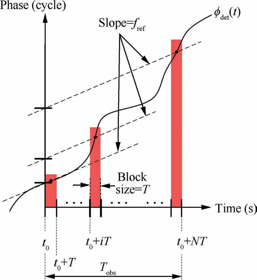
Fig.17 Diagram illustrating the pulse phase tracking concept.

It follows from Eq.(3) that Eq.(2) can be recognized as a function of rSSB（t ）.In practice, we can have a prior information on rSSB（t ）, denoted as ～rSSB（t ）.Then, Eq.(2) can be linearized around～rSSB（t ）, yielding

～rSSB（t ） can be predicted from～rSSB（t0）, obtained by other navigation methods or by propagating from the last epoch, by propagating the orbit dynamics model of spacecraft.147As a consequence, φ（rSSB（t ）） can be expressed as152,153

where φ0and faare unknown.

The SEXTANT team employs the two-dimensional grid search to solve the above problem.152In order to reduce the computational complexity, the parallel computation is employed to accelerate the grid search,154and decouples the estimation of φ0and fafor deep space exploration missions.155fais first searched out and then φ0is estimated by epoch folding.Recently,an on-orbit pulsar timing analysis is proposed to fast estimate φ0,and has been verified by the data from XNAV flight experiments.156

8.Methods to improve navigation performance of XNAV

The principle of XNAV was briefly summarized in Section 4.We first need to find an optimal pulsar combination from a given navigation pulsar database.When the optimal pulsar combination is achieved,both the geometry for a specific navigation mission and the corresponding navigation performance of XNAV in this case can be improved.Moreover, there are many systematic biases within XNAV,which limit the navigation performance of XNAV.Furthermore, the conventional XNAV works with the assumption that a single spacecraft should load at least three X-ray detection systems with large areas to receive the pulsar signal from three directions.This assumption is too ideal for the practical applications.Therefore, in order to improve the navigation performance of XNAV, this section will introduce three types of methods.

8.1.Optimal pulsar combination

This work is usually accomplished by investigating the observability of the navigation system.Most time,the observability is evaluated by the determinant of Fisher Information Matrix(FIM).When there are three pulsars being observed simultaneously, the FIM is derived as157

where niis the direction vector of the ith pulsar and σiis the accuracy of the ith pulse TOA.

Based on Eq.(20), Ref.158 analytically investigates the optimal pulsar combination, and find that the determinant of Eq.(20)will reach its maximum if n1，n2and n3are orthogonal to each other.This conclusion can be extended to a general case where a spacecraft observes N pulsars at the same time.In this case, an optimal pulsar combination should be composed of pulsars with direction vectors orthogonal to each other.

8.2.Systematic biases analysis and compensation

As shown in Eq.(3), the errors within the direction vector of pulsar, positions of planets and the atomic clock recording arrival time of events would affect the navigation performance of XNAV.

For the autonomous navigation in Earth orbits,the impacts of errors within the direction vector of the pulsar,errors within the ephemerides of planets, and clock errors have been analyzed.159–162It is found that those errors vary according to the orbit period of the Earth and thus can be approximated as constants for a navigation process with duration much less than one orbit period of the Earth.This conclusion paves the way for compensating the impacts of those errors.When the XNAV is applied to multi-spacecraft, it has been found that the systematic biases can be eliminated when all the spacecraft observe a common pulsar simultaneously.48

The compensation methods generally consist of three categories, including the augmented-state method,159the timedifferenced method162,163and the H∞/H2filter.164The augmented-state method augments the systematic biases into the state vector,and estimates the systematic biases along with the position and velocity of spacecraft.However, when the number of systematic biases is more than 6, the number of position and velocity, Kalman-type filters employed for estimation might be unstable.Thus, the time-differenced method was proposed.The method employs the difference between pulse TOAs at adjacent time as the measurement for estimation, avoiding the high-dimensional matrices that were involved in the augmented-state method.The H∞/H2filter,originating from the H∞control, derives an upper bound for the systematic biases,and suppresses the impacts of systematic biases by the bounds.However,how to design a proper upper bound is still an open question.

8.3.Integrated navigation

Up to now, the information to be combined with XNAV roughly includes the Earth image information obtained from ultraviolet sensor,165the Doppler velocity measurements relative to the Sun166or the Mars,167the optical measurements on the Mars168,169or the Earth,170,171and the output of inertial navigation system.172,173For the integrated navigation system fusing the star angle information and XNAV, the impacts of direction vector of pulsar,174and the ephemerides errors of Jupiter and other planets175–177have been investigated.The integrated navigation is applied not only to a single spacecraft but also to multi-spacecraft.178,179

The fusion of information from other sources and XNAV is typically achieved by the federated Kalman filter.The federated Kalman filter consisting of parallel filters for each information fuses the outputs of the parallel filters to obtain the final estimation result.Given that the parallel filters work independently, the final estimation result is suboptimal.170A nonlinear kinematic and static filter is derived170,173to overcome the suboptimal fusion of federated Kalman filter.A step Kalman filter structure is designed180to optimally fuse the parallel filters that have greatly different filtering precision.However,the above information fusions work by fusing the pulse phase or TOA and the measurements from the other sources.The achievements of such information fusions are based on the assumption that the pulse phase is obtained.However,as illustrated in Section 7.3,the on-orbit pulse TOA estimation problem has not been well solved.It is a good idea to employ the measurements from the other sources to estimate the pulse phase.171,181

9.Conclusions and future work

In this paper,we review X-ray pulsar navigation(XNAV)systems and the algorithms, and briefly introduce the past, present and future missions with XNAV experiments.This paper focuses on the advances of the key techniques supporting XNAV, including the navigation pulsar database, the Xray detection system, and the pulse TOA estimation, as well as the methods to improve the navigation performance of XNAV.

It can be learned from the review that although several flight experiments on XNAV have been successfully complemented, the wide applications of XNAV still have a long way to go.Further development of XNAV may be pursued from the following aspects:

(1) Designing X-ray detection systems dedicated for navigation.The current X-ray detection systems in space,serve for X-ray astronomy missions, which pursue highquality images or signals with high signal-to-noise ratios.In this case, the volume and weight of an X-ray detection system dominate the payload.However, for a spacecraft with XNAV, the X-ray detection system is just a subsystem of the whole spacecraft.As a consequence,an X-ray detection system dedicated for navigation should be of a small size but have a high detection performance.

(2) Pursuing computationally efficient on-orbit pulse TOA estimation method.Currently, only the pulse TOA estimation for millisecond pulsars have been successfully complemented in orbit.The high flux of Crab pulsar makes the XNAV with small X-ray detection system become applicable,although the stability of Crab pulsar is far less than millisecond pulsars.However, how to quickly estimate the pulse TOA of the Crab pulsar in orbit is an open question.It is because the computational burden in this case is much higher than millisecond pulsars.

(3) Verifying the current navigation algorithms with real Xray pulsar data.Section 8 reviews various navigation algorithms that have been proposed to improve the navigation performance of XNAV.However,most of those algorithms work with simulation data under the assumption that the high-precision pulse ToAs can be obtained.In the algorithms, X-ray detection systems are assumed to have an area of about 1 m2.However,as shown in Tables 2 and 3, such a big area is not easy to achieve in space, even for dedicated X-ray astronomical missions.Furthermore, the flux of a pulsar’s pulsed signal is much less than the background caused by the particles and X-rays from other sources.Thus,the pulse TOA estimation result in the real environment is less accurate than the values assumed in the navigation algorithms.As a consequence,the performance of those navigation algorithms in real cases is quite probably not as good as that in simulations.

Declaration of Competing Interest

The authors declare that they have no known competing financial interests or personal relationships that could have appeared to influence the work reported in this paper.

Acknowledgements

This work was funded by the National Natural Science Foundation of China(No.61703413)and the Science and Technology Innovation Program of Hunan Province, China (No.2021RC3078).