Numerical and experimental investigation of quantitative relationship between secondary flow intensity and inviscid blade force in axial compressors

Chenghu ZHOU, Zixun YUE, Hnwen GUO, Xiwu LIU, Donghi JIN,c,*,Xingmin GUI,c

a School of Energy and Power Engineering, Beihang University, Beijing 100191, China

b AECC Hunan Aviation Powerplant Research Institute, Zhuzhou 412002, China

c Jiangxi Research Institute of Beihang University, Nanchang 330096, China

KEYWORDS

Abstract The secondary flow attracts wide concerns in the aeroengine compressors since it has become one of the major loss sources in modern high-performance compressors.But the research about the quantitative relationship between secondary flow and inviscid blade force needs to be more detailed.In this paper,a database of 889 three-dimensional linear cascades was built.An indicator,called Secondary Flow Intensity(SFI),was used to express the loss caused by secondary flow.The quantitative relationship between the SFI and inviscid blade force deterioration was researched.Blade oil flow and Computation Fluid Dynamics(CFD) results of some cascades were also used to cross-validate.Results suggested that all numerical cascade cases can be divided into 3 clusters by the SFI,which are called Clusters A,B and C in the order of the increasing SFI indicator.The corner stall, known as the strong corner separation, only happens when the SFI is high.Both calculations and oil flow experiments show that the SFI would stay at a low level if the vortex core at the endwall surface does not appear.The strong interaction of Kutta condition and endwall cross-flow is considered the dominant mechanism of higher secondary flow losses, rather than the secondary flow penetration depth on the suction surface.In conclusion, the inviscid blade force spanwise deterioration is strongly related to the SFI.The correlation of the SFI and spanwise inviscid blade force deterioration is given in this paper.The correlation could provide a quantitative reference for estimating secondary flow losses in the design.

Nomenclature A1 inlet axial area A2 outlet axial area AVDR Axial Velocity-Density Ratio c chord cz axial chord D diffusion factor fB normalized inviscid blade force FB inviscid blade force h blade span h- normalized span i incidence angle l length of blade surface element L blade surface curve Ma Mach number n normal vector of blade surface element p static pressure p1 inlet static pressure pps pressure surface static pressure pss suction surface static pressure pt total pressure pt1 inlet total pressure pt2 outlet total pressure R correlation coefficient R2 squared correlation coefficient Rc convergence ratio s blade spacing S Lei’s corner separation size indicator SF inviscid blade force deterioration indicator SI secondary flow intensity tm blade maximum thickness v velocity v1y inlet tangential velocity v2y outlet tangential velocity v1z inlet axial velocity v2z outlet axial velocity y tangential coordinate y+ non-dimensional distance from wall to the first mesh node z axial coordinate γ stagger angle δ boundary layer thickness θ camber angle ρ density ψ loading coefficient ω loss

1.Introduction

Axial compressors of high-performance aero-engines are usually designed with strong three-dimensional flow control, and the secondary flow has attracted wide concerns.1,2Denton3held the view that the loss sources of turbomachinery are complicated, and secondary loss is an important source.The secondary loss exists in the compressor’s three-dimensional passage naturally.Lakshminarayana et al.4,5thought that the interaction between mainstream flow and boundary layer is the main reason for secondary flow loss.

The secondary flow in the compressor stator is complicated.The secondary flow structure is simultaneously affected by the horseshoe vortex, radial secondary flow in the blade surface boundary, and circumferential secondary flow in the endwall.Abdulla-Altaii6and Tang7et al.found that the endwallblade corner flow is affected by the horseshoe vortex.Endwall and blended blade design can be used to control these vortex and loss.8,9Rohlik et al.10interpreted the inner radial flow in stators.The stator surface boundary layer and blade wake usually have lower circumferential velocity than the mainstream flow so that the radial pressure force could surpass the centrifugal force.Roberts et al.11researched the rotor’s radial secondary flow model.By contrast with stators, the centrifugal force of the rotor blade boundary layer is higher than the inner radial pressure gradient.So, the radial secondary flow usually causes a higher secondary flow loss in the rotor’s tip and stator’s hub.The blade surface parameter optimization and bowing blades are usual designs to control radial secondary losses.12,13Circumferential secondary flow, also called crossflow near the endwall, attracted attention too.Johnson and Bullock14thought the imbalance of pressure force and centrifugal force inside the boundary layer is the main reason for cross-flows.As the compressor blade loading rises,the endwall cross-flow grows stronger, affecting 70% of the whole span.15With the development of Three-Dimensional (3D)Computation Fluid Dynamics (CFD), numerical simulations could provide more accurate results about the comprehensive secondary flow.16,17

But for the through-flow calculation, the secondary flow model is still necessary.18,19Researchers in the turbomachinery field have presented many secondary flow models.Because factors for the secondary flow loss are complicated and comprehensive, the model correlations are also various.Ainley and Mathieson20used the drag and lift coefficients, and the secondary flow effect was also included as the secondary drag coefficient.Dunham and Came21used a scale factor of fitting from aspect ratio and flow angle to improve Ainley and Mathieson’s work.Koch and Smith22related the secondary loss to the pressure rise coefficient.Benner et al.23,24fitted the secondary loss with the displacement thickness, passage convergence ratio and penetration depth.In a word, because the causes of the secondary flow are various, different models usually have different independent variables.Still,the common method is to relate the blade geometry and aerodynamic condition.

The inviscid blade force was considered to be related to the secondary flow and the corner separation.Schulz et al.25tested an annular compressor cascade and analyzed the corner separation.The corner static pressure coefficient could be different when the corner stall appears.Hah and Loellbach26studied the corner stall in an axial compressor.The limiting streamline topology of the corner stall was presented both by the CFD and oil flow, showing that the corner stall would lead to the recirculation zone on the endwall surface.Lei et al.27,28used a quantitative indicator to describe the effect of corner separation,and the data can be divided into two sets by the existence of corner stall.A criterion based on the incompressible assumption was presented.Yu and Liu29developed Lei et al.’s criterion with the aspect ratio as a new factor.The researches revealed that the inviscid blade force is related to the secondary flow and separation.But the quantitative relationship between the Secondary Flow Intensity (SFI) and inviscid blade force deterioration has not been given.Compressibility was also not considered in the criteria.

In this paper, numerical and experimental methods were used to reveal the dominant mechanism of corner separation.889 compressor stator cascades were computed and 4 cascades were tested.889 numerical cases were used to build the database, and 4 cases with CFD and oil flow result were used to cross-validate the result.The quantitative relationship between SFI and inviscid blade force deterioration was given.

2.Numerical setting and experimental facility

2.1.Variable definitions

The definition of loss ω is the total pressure loss coefficient:

where pt1and pt2are the inlet and outlet total pressure,and p1is the inlet static pressure.

To describe the Secondary Flow Intensity(SFI),the following indicator SIis defined:

where ωaverageis the mass average loss across the whole span,and ωh-=0.5is the loss at the middle span, as shown in Fig.1.This indicator can also be used as the coefficient in the through-flow calculation to include secondary flow loss.Besides, the SFI indicator can also work as the distinguishing criterion for building a machine learning loss model19.

The secondary flow usually affects the spanwise distribution of the inviscid blade force,as shown in Fig.2.The method of quantifying the size of corner separation, presented by Lei et al.27,28, uses the following equation:

Fig.1 Definition of Secondary Flow Intensity (SFI).

Fig.2 Pressure distribution at different spans.

where ψ is the Zweifel loading coefficient from Dixon30:

where z is the axial coordinate,czis the axial chord length,ppsis the static pressure of the pressure surface,and pssis the static pressure of the suction surface.

The spanwise inviscid blade force is calculated from the pressure difference between the pressure surface and the suction surface.But in the calculation in Eq.(4),the inviscid blade force is not a vector with an axial component.And the axial component is affected by the stagger angle and secondary flow.The inviscid blade force direction could change apparently if the corner stall happens.

In this paper, a new dimensionless quantitative indicator is presented to describe the deterioration caused by corner separation:

The physical meaning of SFis the inviscid blade force difference between the 50% and 10%span.The vector fBis defined to build the dimensionless indicator as follows:

For a cascade blade surface curve at one span L, the inviscid blade force is defined as:

where p is the blade surface static pressure, and dn is the normal vector of a blade surface element.The force FBis a physical quantity with the unit different from the pressure,and it is related to the length of the blade surface.Compared with the traditional method of Eq.(3), the indicator of Eq.(5) is more accurate to describe blade force deterioration.The force direction should be considered when dealing with the inviscid blade force deterioration.The integral definition ofused by SFcontains the effect of the axial force, but the integralused by S is the circumferential blade force.The flows in most cases are compressible in this paper.Thus, the criteria with incompressibility by Lei27,28and Yu29et al.are not used.Lieblein’s diffusion factor D is an important dimensionless variable to describe blade profile loading.31The definition is as follows:

Fig.3 Schematic diagram of inviscid blade force calculation.

where v1and v2are the inlet and outlet velocity,v1yand v2yare tangential velocity at inlet and outlet, s is the tangential spacing of blades, and c is the blade chord.

2.2.Setting of numerical database

Twenty 3D cascades were created with Controlled Diffusion Airfoil (CDA) thickness distribution.32The variable ranges are listed in Table 1.The stator geometry used in the compressor is designed with prior knowledge.For example, the maximum camber angle and stagger angle are usually higher in the stator’s shroud section than the hub section.The aspect ratio and axial area convergence ratio could decrease as the stage number grows.The variable combination was taken from thestator geometry of Energy Efficient Engine’s high-pressure compressor’s ten stages, and a 9.271-pressure-ratio compressor’s first three stages were used as references.33,34

Table 1 Database specifics.

The stagger γ, camber θ, solidity s/c and max thickness/-chord tm/c are related to the profile loss.The aspect ratio h/c and convergence ratio Rc=A1/A2are set to account for the convergence effect of passages, and these ratios are also used to relate the secondary loss.20,23,24A1and A2are the axial area of the inlet and outlet.The 20 profiles are shown in Fig.4.The incidence angle i and inlet Mach number Ma1are usually used as critical independent variables to describe off-design conditions.35The inlet total pressure was set to 101325 Pa for all cases.As the incidence and backpressure changed, the inlet Mach number of all cases was unique for each case.The Reynolds number is not set as a variable because the secondary flow loss is negligibly affected by the Reynolds number in the range from 105to 106,according to Horlock and Lakshminarayana’s work.4

The Navier-Stokes (N-S) equation with Jameson central scheme was chosen to solve the steady Three-Dimensional(3D) flow fields.36The Spalart-Allmaras turbulence model was applied for fast solving and acceptable accuracy.37The NUMECA v9.0–3 was the flow solver.Two planes, one with the axial location at z/cz=-0.1 and the other at z/cz=1.1,were used to extract inlet and outlet data.

The blade-to-blade grid topology is O4H, as shown in Fig.5.The number of the spanwise layer is 125.The typical grid parameter of one stage is shown in Table 2.The generalized Richardson extrapolation was used to evaluate the grid independence.38To achieve grid independence for SFI,the grid number level was chosen as 1.24 million nodes, as shown in Fig.6.The same grid topology was used for the other 19 blades,and the values of skewness,aspect ratio and expansion ratio were within a range of 10% from Table 2.

The reference y+value of the Spalart-Allmaras turbulence model in NUMECA is 1–10,and the typical result of y+distribution is given in Fig.7.The wall function was not used.

In his book The Great Lili, Carlton Jackson records that Nazi19 propaganda minister Josegh Goebbels detested20 “Lili.” He wanted morale-boosters like “Bombs on England”. He ordered the original master copy of Lale Andersen s recording17 destroyed. When Stalingrad fell in January 1943, after 300,000 German soldiers had been killed, Goebbels banned the song entirely21, saying that “a dance of death roamed throughout its bard22.”

2.3.Cross-validation of numerical and experimental results

A cascade test and corresponding numerical computation were carried out to cross-validate the quantitative relationship.The test cascade is manufactured using the following parameter in Table 3.

The midspan loss distribution of this database is given in Fig.8.The numerical database matches Rechter et al.’s32experiment data if the inlet Mach number is lower than 0.8.In Rechter et al.’s32data, the Axial Velocity Density Ratio(AVDR) at the middle span was kept constant at 1.1 in the experiment, and the incidence was maintained at 0°.The AVDR is defined as follows:

For compressor cascades, the AVDR is a variable to evaluate how the axial flow area is affected at the middle span.In the numerical database of this paper, the AVDR is not a controlled constant.Because the profile geometry and aerodynamic condition are different, the validation of the numerical database is qualitative.

Fig.4 Definition of blade profiles and convergence ratio.

Fig.5 Mesh topology.

Table 2 Grid information.

The test facility of compressor cascades supported the test of low-speed cascades.Previous results from this test facility can be found in Liu et al.’s work.39,40The oil flow test was applied in 2 cases with incidence angles at 0° and +7°.The inlet temperature was 299.4 K, and the Reynolds number was 1.67 × 105.The CFD surface limiting streamlines and oil flow results match well, as shown in Fig.9.Both in the experiment and numerical calculation, no corner stall was found, as there was no strong backflow causing a vortex core at the endwall surface.With this cross-validation, blade surface pressure results of CFD were used to calculate the spanwise inviscid blade force.

3.Results and discussion

3.1.Correlations of SI and SF

There exists a strong correlation between SFI SIand spanwise inviscid blade force deterioration indicator SFas follows:

This linear regression of numerical data gives the correlation coefficient R at about 0.83, as shown in Fig.10.

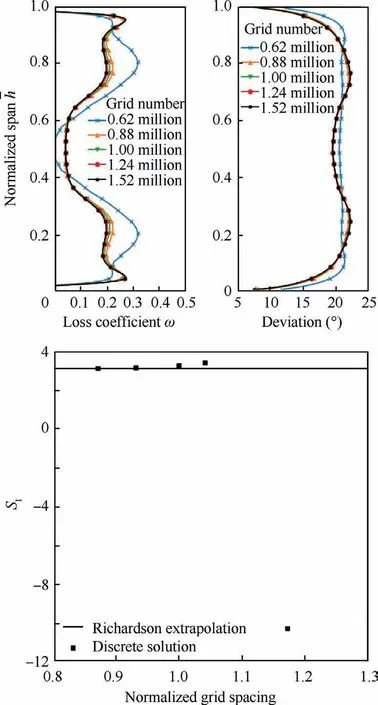
Fig.6 Results of grid independence study.

The Gaussian kernel density estimation gives the data density distribution in the space spanned by （SF，SI）,and the result is shown in Fig.11.There are 3 clusters in the numerical database.Four experimental cases are all in Cluster B.An offset of experimental data is found from the numerical data.

A possible reason for the higher SFin the experiment data is that the experimental boundary layers are thicker than the numerical database.The relative boundary layer thicknesses δ/h of numerical data are 4%-5%, but the values are about 10%-15%in the experimental cases.Here the δ is the boundary layer thickness, and the h is the blade span.As shown in Fig.12, the boundary layer thickness and loss of 4 cases with experiment data are higher than the numerical case.And the span affected by secondary flow is relatively higher than in the experiment.

Fig.7 Validation of y+.

Table 3 Configuration of test cascades.

Because the SFis defined with the inviscid blade force difference between the middle span section and 10%span section,the higher SFis found in experimental data.The limiting streamlines and spanwise loss distribution are shown in Figs.13 and 14.

Cluster A has the center with SIaround 1.0 and SF<0.It indicates that the average loss ωaverageis almost equal to the loss in the middle span ωh-=0.5.According to the definition, if SF<0, a larger inviscid blade force magnitude ｜fB｜could be found at the 10%relative span rather than at the 50%relative span.The flow in the 10% relative span could be affected by the endwall boundary, and shocks would not be as strong as in the middle span.The cases with SF<0 are mainly in Cluster A,whose secondary flow intensity SIis about 1.0.The 2D loss is dominated by the total loss of Cluster A,rather than the secondary loss.Separation lines are found across the blade surface.For cases in Cluster A, the inlet Mach number is higher than that of the other 2 clusters.Some cases have shocks if the inlet Mach number goes high, while some cases have negative incidence and pressure surface separation.

Cluster B has the highest data density,with a cluster center around （SF，SI）= （0.025，1.4）.The middle span loss of Cluster B is usually at a low level, and the secondary flow would not affect the whole span.For cases in Cluster B,a corner separation could be found.There may exist a deep secondary flow penetration in the blade suction surface as shown in Fig.13,but the volume of the corner separation bulb is relatively small,resulting from the weak SFI.An important fact is that the endwall surface does not have a vortex core at the corner area in Cluster B.Four experimental test points also agreed with this feature, whose nearest cluster is Cluster B.

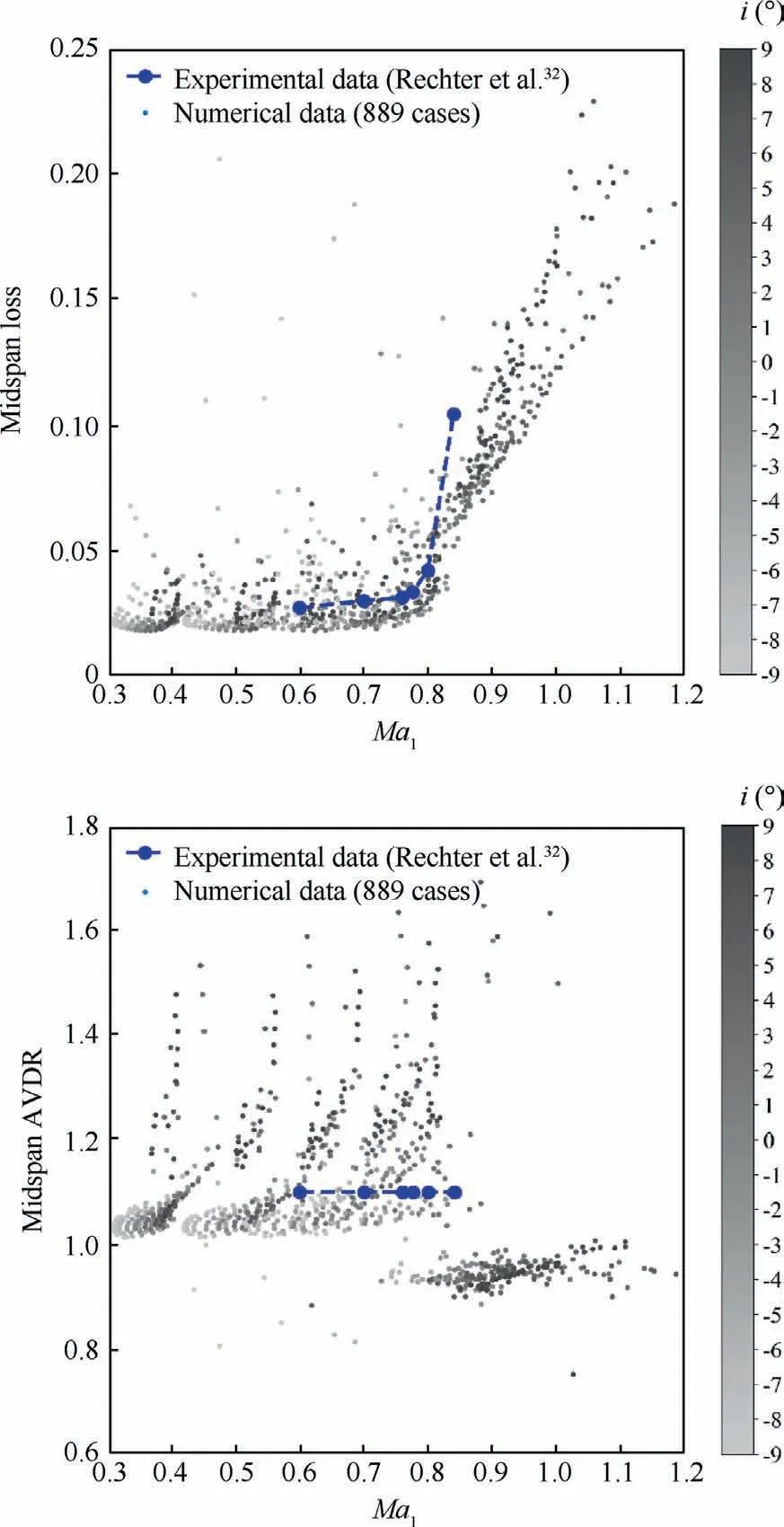
Fig.8 Numerical and experimental data.

Cluster C mainly consists of cases with the corner stall,which means the high secondary flow effect on spanwise loss.The maximum density of Cluster C is smaller, and data are more scattered.As shown in Fig.14, though the secondary flow intensity is strong in these cases, the middle span loss remains at a low level.Cases in Cluster C have a strong backflow on the endwall surface,compared with cases in Cluster B.And it would create a vortex core connecting the endwall and blade suction surface, causing a corner stall bulb.The volume of corner separation would grow apparently if this vortex core was built.Similar findings were given by Taylor41and Kan42et al.Their work also reveals that the endwall limiting streamline topology would produce a focus point if the corner stall happens.The secondary flow loss would rapidly grow once exceeding a critical condition.

Fig.10 Linear regression prediction.

Fig.11 Three cluster centers in kernel density estimation.

Fig.12 Spanwise loss of numerical and experimental data.

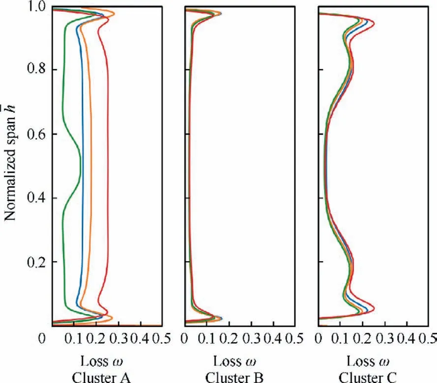
Fig.14 Spanwise loss distribution.

3.2.Relation of SI and preliminary design parameters

The cases with higher incidence angle and medium inlet Mach number are found easier to form the secondary flow pattern in Cluster C, whose secondary intensity is high, as shown in Figs.15 and 16.Most cases in Cluster C have the inlet Mach number around 0.8.If the inlet Mach number is high,the separation tends to be two-dimensional,whose SFI would be low.And when the inlet Mach number is low,the SFI would stay in Cluster B around 1.4, whose corner separation is not considered as the corner stall with the strong separation.

In the trailing edge of the compressor cascade in Cluster C,the Kutta condition would keep in the middle span, and the loss would keep low simultaneously.But the stream velocity is lower in the endwall boundary layer, and the endwall cross-flow is stronger.In the cases of Cluster C,the free stream velocity magnitude is high enough to form the pressure gradient from the pressure surface toward the suction surface.Meanwhile,the incidence is positive with enough aerodynamic loading and endwall tangential momentum.The interaction of Kutta condition and endwall cross-flow gives the corner stall flow topology, causing the high SFI and spanwise inviscid blade force deterioration.

The results of Figs.17 and 18 show that the database stays in the pattern of 3 clusters.Cluster A has a relatively high inlet Mach number, Cluster B has the low one, and Cluster C has the medium one.The middle span diffusion factor almost does not affect the SFI in the flow patterns of Cluster A and Cluster B.In Cluster C, the incidence, inlet Mach number and diffusion factor could result in a secondary loss increase.The cases with the highest SFI usually have the upper bound ofat 0.4.It indicates that the blade load at the middle span would not increase when the corner stall happens.

Fig.13 Patterns of limiting streamlines.

Fig.15 Effect of incidence angle on SI and SF (circle dots for numerical data; square dots for experimental data).

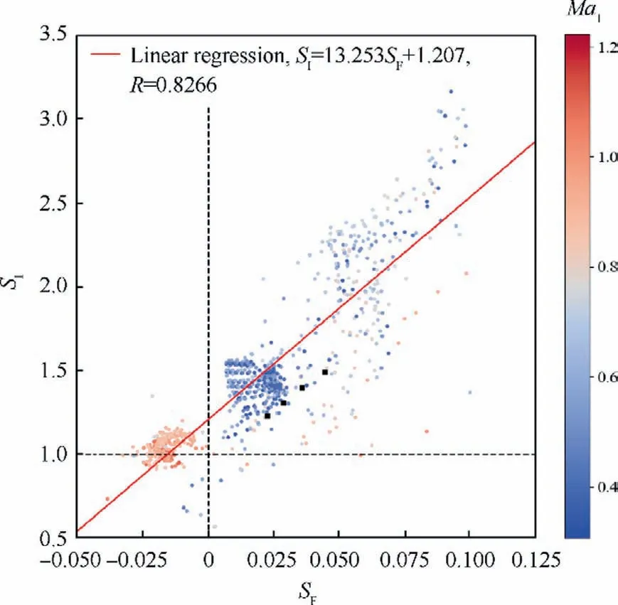
Fig.16 Effect of inlet Mach number Ma1 on SI and SF (circle dots for numerical data; square dots for experimental data).

In Fig.17, the diffusion factor at the midspan would increase as the incidence increase inside the clusters.Both positive and negative incidences can be found in all three clusters.And the diffusion factor at midspan would grow as the incidence grows in Cluster C.In Clusters A and B, the secondary flow intensity stays around 1.0 and 1.4 regardless of the effect of diffusion factor and incidence, showing that the sudden change of the secondary flow intensity usually comes from

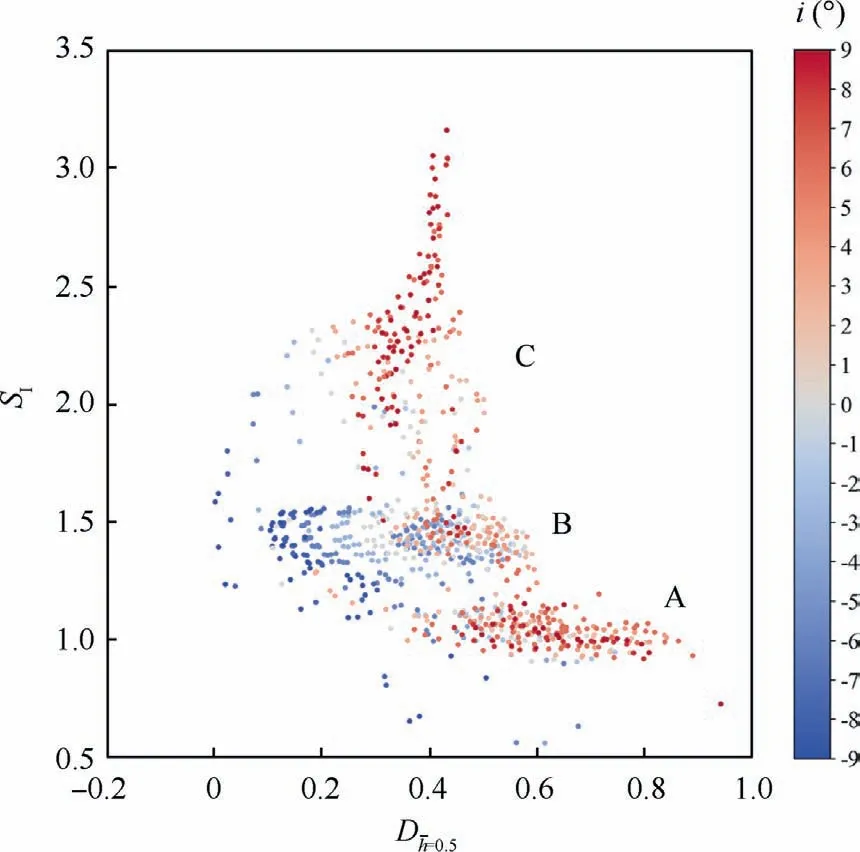
Fig.17 SI vs diffusion factor D with different incidence angle i.

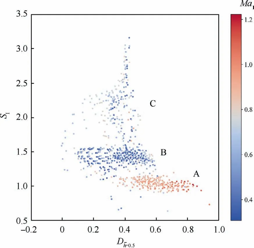
Fig.18 SI vs diffusion factor D with different inlet Mach number Ma1.

the change of flow topology structure.In Fig.18,three clusters have three different inlet Mach number levels.Most cases in Cluster A have the inlet Mach number over 0.8, and the loss is mainly compounded by the 2D loss.In Cluster B, the inlet Mach number of most cases is lower than 0.6.The diffusion factor at the middle span and inlet Mach number do not strongly affect the secondary flow intensity inside Cluster B.With the above analyses, a polynomial correlation with R2=0.848 is presented for the preliminary design to predict the secondary flow intensity.The expression is as follows:

Table 4 Coefficients of constant and first degree.

Table 5 Coefficients of second degree.

where xiare the variables as follows:

The coefficients are shown in Tables 4 and 5.

4.Conclusions

In this paper, a numerical database was built to research the quantitative relationship between the secondary flow intensity SIand inviscid blade force deterioration SF.The oil flow and CFD results were used for cross-validation.The flow topology and data distribution were analyzed.Spanwise loss and inviscid blade force were used to calculate the SIand SF.The following conclusions can be drawn:

(1) There are 3 clusters found in the secondary flow patterns.In Cluster A, the total loss is dominated by 2D loss.In Cluster B, the secondary flow intensity is stronger than in Cluster A, but the corner separation is not open.The corner separation in Cluster B would not arouse high secondary flow intensity.In Cluster C, the secondary flow with corner stall would affect more span than the other two clusters while the loss at the middle span keeps low, causing a higher SFI value.

(2) There is a strong positive correlation between SIand SFwith a correlation coefficient of about 0.83.A correlation with the preliminary design variable was presented.The correlations could provide a quantitative reference for the early estimate of secondary flow losses in the design.

(3) The high secondary flow loss,related to the corner stall,results from the strong interaction of Kutta condition and endwall cross-flow.High secondary loss usually happens at the medium inlet Mach number and positive incidence conditions.The flow topology could be different since the endwall could form a saddle and focus pair.This topology is a result of the strong reverse flow in the flow passage.

Declaration of Competing Interest

The authors declare that they have no known competing financial interests or personal relationships that could have appeared to influence the work reported in this paper.

Acknowledgements

This research was supported by the National Science and Technology Major Project, China (Nos.2017-I-0005-0006 &2019-II-0020-0041).