μ-Synthesis control with reference model for aeropropulsion system test facility under dynamic coupling and uncertainty

Jishui LIU, Xi WANG, Xi LIU,*, Meiyin ZHU, Xitong PEI,Song ZHANG, Zhihong DAN

a School of Energy and Power Engineering, Beihang University, Beijing 100191, China

b Zhongfa Aviation Institute, Beihang University, Hangzhou 311115, China

c Research Institute of Aero-Engine, Beihang University, Beijing 100191, China

d Science and Technology on Altitude Simulation Laboratory, AECC (Aero Engine Corporation of China) Sichuan Gas Turbine Establishment, Mianyang 621703, China

KEYWORDS

Abstract Due to the dynamic coupling and multi-source uncertainties, it is difficult to accurately control the pressure and temperature of the Aeropropulsion System Test Facility (ASTF) in the presence of rapid command and large disturbance.This paper presents the design of μ-synthesis control to solve the problem.By incorporating the pressure ratio into the linear equation of the control valve, the modeling error of ASTF in the low frequency range is effectively reduced.Then, an uncertain model is established by considering various factors,including parameter variations,modeling error in the low frequency range,unmodeled dynamics,and changes in the working point.To address the dynamic coupling,a diagonal reference model with desired performance is incorporated into μ-synthesis.Furthermore, all weighting functions are designed according to the performance requirements.Finally, the μ-controller is obtained by using the standard μ-synthesis method.Simulation results indicate that the μ-controller decouples the pressure and temperature dynamics of ASTF.Compared with the multivariable PI controller, integral-μ controller, and double integralμ controller,the proposed μ-controller can achieve higher transient accuracy and better disturbance rejection.Moreover, the robustness of the μ-controller is demonstrated by Monte Carlo simulations.

1.Introduction

Aeropropulsion System Test Facility (ASTF) provides a ground-test environment for aircraft engines.1By controlling the pressure and temperature of the airflow supplied to the engine, ASTF can simulate flight conditions (i.e., altitude and Mach number) to test the performance of the engine.1–3Generally,ASTF is used to simulate fixed or slowly changing flight conditions.4However, with the development of highperformance engines, ASTF needs to have the capability of conducting ‘‘maneuvering flight” tests.This implies that the engine can accelerate or decelerate arbitrarily, and the flight conditions will change rapidly.5In other words, ASTF must ensure rapid transient responses of controlled pressure and temperature while suppressing large disturbances.6However,the pressure and temperature dynamics of ASTF are strongly coupled, which makes it difficult to accurately regulate the pressure and temperature simultaneously.Moreover, the multi-source uncertainties caused by various factors (e.g.,parameter variations, modeling error in the low frequency range, unmodeled dynamics, and changes in the working point)further degrade the performance of the closed-loop system.Therefore, the controller must deal with dynamic coupling and uncertainties to ensure good performance and robustness.

First of all,it is necessary to establish a model of ASTF for controller design.In Refs.7,8, the relationship between the valve opening and the control command was established based on valve characteristics, mass balance, and energy balance.Generally,this relationship is used for open-loop control.Luppold et al.2proposed an identification algorithm to estimate the system model,which can be used to update the parameters of the controller.In Refs.6,9, the pressure dynamic of ASTF was modeled as a double integral system with generalized disturbance.Although this method requires less knowledge about the system dynamics, it increases the burden of the controller to deal with larger uncertainties.More generally,Zhu et al.10,11adopted the state-space method to establish a model for ASTF, which is more suitable for the design of model-based controllers.However, the linear model of the control valve neglects the influence of the pressure ratio on the mass flow,which leads to large modeling errors.As a result, the designed controller has to sacrifice control performance to ensure robustness against large modeling errors.

The controller for ASTF aims at precise regulation of pressure and temperature.To improve the control accuracy of pressure, Refs.2,8 introduced feedforward control into the closed-loop system.However,the feedforward control requires high-precision valve characteristics, depending on lots of experiments.12,13Zhang et al.14proposed a fuzzy-PID controller to reduce the requirement for model accuracy.Another method is to design a PD controller with an extended state observer, which can compensate for uncertainties and disturbances.6,9These single-variable control methods effectively improved the control accuracy of pressure.When the pressure and temperature were regulated simultaneously,the decentralized PID controller was naturally adopted.7However, due to the neglect of the strong coupling between pressure and temperature dynamics,the system responses were not satisfactory.In Ref.15,a multivariable PI controller based on linear quadratic optimization showed good tracking performance in the numerical simulation of ASTF, which demonstrated the advantage of the multivariable controller in dealing with coupling.However, this method requires an accurate model of ASTF.Therefore,Zhu et al.16designed a multivariable PI controller based on regional pole placement to improve the robustness of the closed-loop system.Nevertheless, the range of uncertainties addressed by this method is not clear.Thus,a large number of steady-state controllers need to be scheduled to control the pressure and temperature in the whole working envelope.It is well known that the H∞optimization approach is an effective robust design method for uncertain systems.17However, the H∞approach only guarantees nominal performance and robust stability against unstructured uncertainties.17,18Therefore, the μ-synthesis approach based on the structured singular value was developed to achieve robust stability and robust performance.19–21Moreover, the μ-synthesis is constructed based on the H∞approach and μ-analysis.It is less conservative than the H∞approach for structural uncertainties.22–24μ-synthesis control has been adopted in many research fields.25–30In Refs.10,31, robust μ-synthesis was adopted for the multivariable control of ASTF.Based on this,Zhu et al.11proposed a Linear Parameter Varying(LPV)based μ-synthesis method for ASTF.Although this method ensures the servo performance of ASTF, μ-controllers need to be designed to have the same order.This makes the Structured Singular Value (SSV) often greater than 1, thereby reducing the robust performance margin.17In addition, the dynamic coupling may seriously deteriorate the system response in the presence of rapid command and large disturbance.In Ref.32, the robust optimal adaptive control adopted a reference model to specify the desired performance, thereby decoupling the pressure and temperature dynamics.However, it can only deal with matched uncertainties.

Motivated by the above investigations, this paper proposes a reference model-based μ-synthesis control with regard to the dynamic coupling and multi-source uncertainties of ASTF.The main contributions of this paper are summarized as follows:

(1) The modeling error in the low frequency range is effectively reduced by improving the linear model of ASTF.This is beneficial to model-based controller design.

(2) Compared with previous studies, this paper systematically describes and deals with multi-source uncertainties in a single control framework.

(3) In the presence of rapid command and large disturbance, the proposed approach provides an effective solution for the accurate control of the coupled system variables (i.e., pressure and temperature).

The rest of this paper is organized as follows.The improved modeling method of ASTF is introduced in Section 2.Section 3 provides the detailed design of μ-synthesis control, including the analysis of multi-source uncertainties, the quantification of performance, and the selection of weighting functions.Section 4 presents the numerical simulation results.The discussions are provided in Section 5.Finally, the conclusions are given in Section 6.

2.Modeling of ASTF

ASTF is composed of control valves, pipeline, mixer, flow straightener subsystem, air source, etc., as shown in Fig.1.33The airflows provided by the air sources are mixed in the mixer and the flow straightener subsystem.Then,the mixed airflow is supplied to the aircraft engine.The parameters (i.e., pressure and temperature) of air source 1 are different from those of air source 2.By regulating the opening of control valves, the mass flow of two airflows can be changed to control the pressure and temperature of the airflow at the export.

Fig.1 Schematic diagram of ASTF.33

2.1.Nonlinear model of ASTF

To evaluate the performance of the designed controller, the nonlinear model of ASTF is used for subsequent simulations.The nonlinear model is established based on the multi-volume modeling method, which regards the control valves and the flow deflectors as throttling devices.Then, the ASTF can be divided into four volumes (see the dash-dotted line in Fig.1).Each volume can be modeled to simulate the pressure and temperature dynamics of the compressible airflow,wherein the heat transfer of the pipeline is considered.The throttling device is modeled according to the flow characteristics obtained from the experimental data and flow field simulation data.In addition, the mechanism model of the valvecontrolled hydraulic cylinder is adopted to simulate the dynamics of the actuator.The detailed description of the nonlinear model can be found in Ref.33.

2.2.Linear model of ASTF

To establish a linear model,the ASTF is considered to be composed of two control valves and a lumped volume (see the dashed line in Fig.1).

2.2.1.Linear model of lumped volume

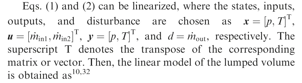
The lumped volume of ASTF includes two inlets and one outlet, as shown in Fig.2.When neglecting the heat transfer and gravitational potential energy, the pressure and temperature dynamics of the lumped volume can be described by10

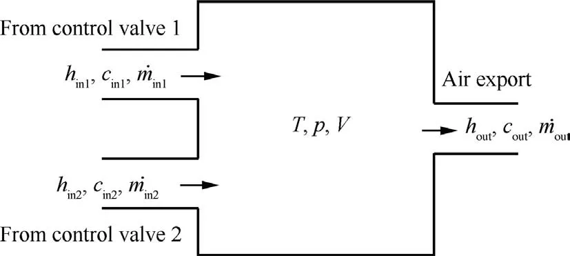
Fig.2 Lumped volume model of ASTF.

where ˙min1,hin1,and cin1represent the mass flow,enthalpy,and velocity of the airflow from control valve 1, respectively; ˙min2,hin2,and cin2represent the mass flow,enthalpy,and velocity of the airflow from control valve 2, respectively; ˙mout, hout, and coutrepresent the mass flow, enthalpy, and velocity of the airflow at the export, respectively; T, p, and V are the temperature, pressure, and volume of the lumped volume,respectively;R is the gas constant;cpis the specific heat at constant pressure.

2.2.2.Linear model of control valve

The mass flow regulated by the control valve can be written as34

where φ and Amaxare the flow coefficient and the maximum flow area of the control valve,respectively;p1and T1represent the upstream pressure and upstream temperature of the control valve, respectively; Vpis the valve opening with a range of 0°–90°.

When linearizing Eq.(4),previous studies only focus on the relationship between mass flow and valve opening.3,16,31The model is expressed as

Both p1and T1are constant values, because the upstream component of the control valve is stable air source.However,the flow coefficient φ is related to the pressure ratio π(i.e.,the ratio of the downstream pressure p2to the upstream pressure p1) and the valve opening, as shown in Fig.3.When the control valve works in area 1(see the solid line in Fig.3),the flow coefficient is less affected by the valve opening and the pressure ratio.Then, φ can be approximated as a constant value, and Eq.(5) is reasonable.When the control valve works in area 2 (see the dashed line in Fig.3), the flow coefficient is less affected by the valve opening.However, the flow coefficient has a negative correlation with the pressure ratio.Then, the modeling error of Eq.(5) may be very large.

Since the influence of valve opening on flow coefficient can be neglected, a fixed valve opening (see Line 1 in Fig.3) is selected to obtain the relationship between the flow coefficient and the pressure ratio (see Fig.4).Actually, we only need the derivative of the flow coefficient with respect to the pressure ratio (i.e., Eq.(6)), which can be obtained by the piecewise approximation shown in Fig.4.

Considering the pressure ratio, Eq.(4) can be linearized into Eq.(7) at the steady-state point.

where

According to Eqs.(7)and(8),the linear model composed of control valve 1 and control valve 2 is written as

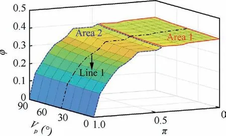
Fig.3 Flow coefficient of control valve.

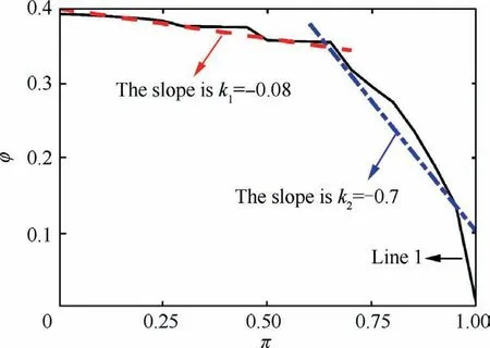
Fig.4 Relationship between flow coefficient and pressure ratio.

where π1, Vp1, Kv1, and pg1represent the pressure ratio, opening, flow gain, and upstream pressure of control valve 1,respectively; π2, Vp2, Kv2, and pg2represent the pressure ratio,opening, flow gain, and upstream pressure of control valve 2,respectively.

Moreover, according to Eq.(5), the linear model established by the previous method is

2.2.3.ASTF modeling

Define the vector v=[Vp1Vp2]T.Then,the improved ASTF’s model given by Eqs.(3) and (9) is written as

where

According to Eqs.(3)and(10),ASTF’s linear model established by the previous method can be written as

where

To make the design of the controller easier,Gp(s)is normalized.10The reference values of pressure,temperature,opening,and mass flow used for normalization are p0, T0, Vp0, and ˙m0,with

Subsequently, all systems and signals are normalized.We would slightly abuse the notation by using Gp(s) to denote the normalized plant of ASTF.

From Apand, it can be seen that the dynamics of the linear model are changed by introducing the pressure ratio into the linear equation of the control valve.Actually,this improvement effectively reduces the modeling error in the low frequency range, which can be verified by the following comparison.

The pressure and temperature of air source 1 are set at 135 kPa and 300 K,respectively.The pressure and temperature of air source 2 are set at 120 kPa and 230 K,respectively.The mass flow of the airflow at the export is 100 kg/s.When the airflow pressure and temperature at the export are stabilized at 90 k Pa and 280 K, we can obtain the linear models of ASTF using different methods, including the improved method (i.e.,Eq.(11)), the previous method (i.e., Eq.(13)), and the frequency sweeping experiment.Fig.5 shows the frequency domain characteristics of these models.

From Fig.5,the improved method effectively reduces modeling errors in the low frequency range.Moreover, the improved model is a linear low-order model.Therefore, the modeling accuracy in the high frequency range is still not high.However, these residual modeling errors can be addressed in the subsequent μ-synthesis design.

3.μ-Synthesis with reference model

3.1.Analysis of uncertainties

From the above discussion,the improved model still has modeling errors and unmodeled dynamics.In addition, the working envelope of ASTF is wide, and the dynamic characteristics of ASTF at different steady-state points are quite different.In this section,these multi-source uncertainties are modeled and quantified to perform the μ-synthesis design.

The working envelope of ASTF is shown in Fig.6.3The designated steady-state point (see the triangle in Fig.6) is taken as the nominal design point, which is modeled in the form of Eq.(11) with

Then, ASTF can be described as a model with multiplicative uncertainty in the whole working envelope, that is

where ‖∙‖∞represents H∞norm.

Fig.5 Frequency domain characteristics of ASTF at steady-state point.

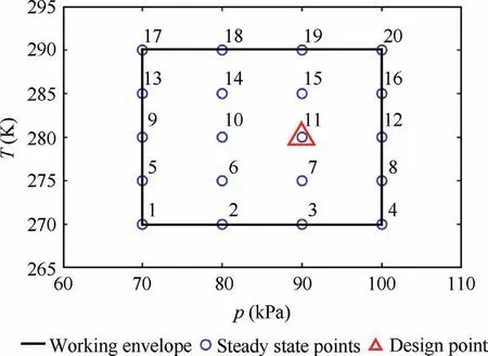
Fig.6 Working envelope of ASTF.

The weighting function describes the maximum relative error between the actual working point and the nominal design point.Here,select 20 steady-state points in the working envelope (see Fig.6), and construct the magnitude responses (see the dashed line in Fig.7) of the relative errors between the steady-state points and the nominal design point.Then, the weighting functions can be determined according to the upper bound of these magnitude responses.The uncertain plant（s）(i.e.,Eq.(19))is a transfer function matrix,which contains six unstructured uncertainty blocks.Strictly speaking,six weighting functions are required to build the uncertain plant（s）.Generally,this makes the controller design more difficult.However, for all inputs and the disturbance, the magnitude responses of the pressure dynamic are basically the same (see Fig.5).And the same is true of the temperature dynamic.Therefore,we can apply the same weighting function to some elements of（s）, as shown in Fig.7.

From Fig.5,we can see that the linear model has high accuracy in the middle and low frequency range (w < 50 rad/s).Hence, the uncertainty weighting function should be close to the upper bound of these relative errors.Because of the unmodeled (usually high-frequency) dynamics, the weight gradually increases with the increase of frequency.As a result,the uncertainty weighting functions are chosen as

W1(s) implies that the uncertainty is 35% in the low frequency range, 100% at the frequency of 50 rad/s, and 800%in the high frequency range.For temperature dynamic,neglecting heat transfer leads to larger uncertainty.Then,W2(s) represents that the uncertainty is 65% in the low frequency range, 100% at the frequency of 50 rad/s, and 1000% in the high frequency range.

Based on the above uncertainty weighting functions,ASTF(i.e., Eq.(19)) can be simplified as a plant with output multiplicative uncertainty, that is,

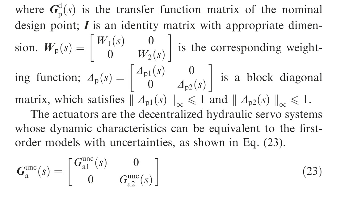
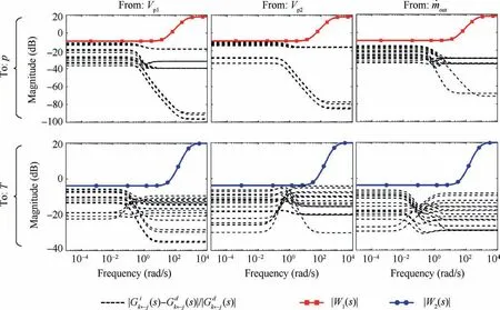
Fig.7 Relative errors between steady-state points and nominal design point.（s） is the transfer function of i-th steady state point from j to k, and i = 1, 2,..., 20.

3.2.Performance requirements

The block diagram of μ-synthesis with a reference model is shown in Fig.9, in which r, vc, v, d, y, ya, ym, yref, e, dist, n,zu, and zprepresent the command, controller output, control input, low-frequency disturbance, nominal plant output,actual plant output, measurement signal, desired trajectory,tracking error, disturbance at arbitrary frequency, noise, control signal evaluation, and tracking performance evaluation,respectively.The objective is to design a μ-controller K(s) to ensure the robust stability and robust performance of the closed-loop system with uncertainties.

3.2.1.Disturbance and noise

The disturbance d of ASTF refers to the change of intake airflow of the aircraft engine.The normalized disturbance dist is shaped by the weighting function Wd(s), which should be frequency-dependent.The rapid acceleration time or deceleration time of the engine is about 5 s.Therefore, the magnitude of Wd(s) should maintain constant at low frequency and decrease 20 dB/decade for frequencies larger than 0.8 rad/s,i.e.,

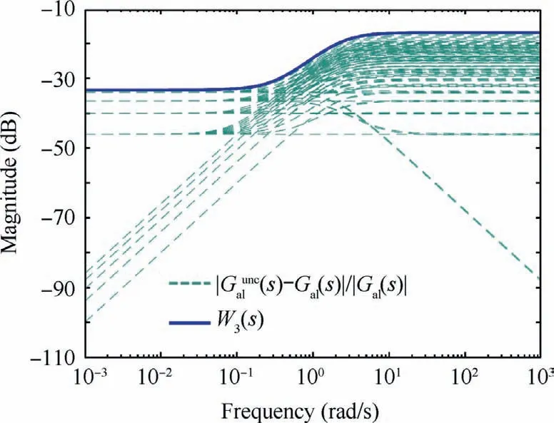
Fig.8 Approximation with multiplicative uncertainty.

where kdis an adjustable gain coefficient.The larger the gain kd, the better the disturbance rejection performance over the frequencies less than the corner frequency.In this paper, kdis taken as 0.8, which can also be interpreted as that the maximum allowable disturbance is 80% of the reference value ˙m0.

The measurement fed back to the controller includes sensor noise, which can be characterized by the additive signal.The noise n is a normalized signal.The noise levels of pressure and temperature are about 0.2 kPa and 0.3 K, respectively.Hence, we use 0.2/p0and 0.3/T0to model broadband sensor noise, that is,

3.2.2.Design specifications

The pressure and temperature dynamics of ASTF are coupled.Thus, a diagonal reference model Mref(s) is selected to prescribe the desired dynamic and suppress the interaction between the two channels, as shown in Eq.(29).

Remark 1.M0(s)is set as a second order lag.And the rise time tr, overshoot Mp, and settling time tsof its step response are quantified by Eqs.(30),(31),and(32),respectively.35,36Then,ξ and wncan be determined by the time-domain specifications(i.e., tr, Mpand ts) of the closed-loop system.

Remark 2.To simulate the flight mission profile of the aircraft engine, ASTF will be given ramp commands of pressure and temperature.10,11For any ramp commands rp(t) and rT(t), the reference model Mref(s) consisting of two same second-order systems has predictable responses(i.e.,yref,p(t)and yref,T(t)),as shown in Fig.10.35,36It can be known that the command pair{A1, B1} at time t1(except the initial stage) can always be tracked at the same rate by the response pair {A3, B3} at time t3,which implies that ASTF can still effectively test the engine after the time interval Δt.However, the traditional control method does not specify the same dynamics of pressure and temperature,which makes it difficult for the response pair{A2,B2} to reproduce the command pair {A1, B1}.As a result,ASTF cannot effectively conduct performance test on the engine,because the pressure and temperature must be matched to accurately reflect the required flight conditions of the engine.4

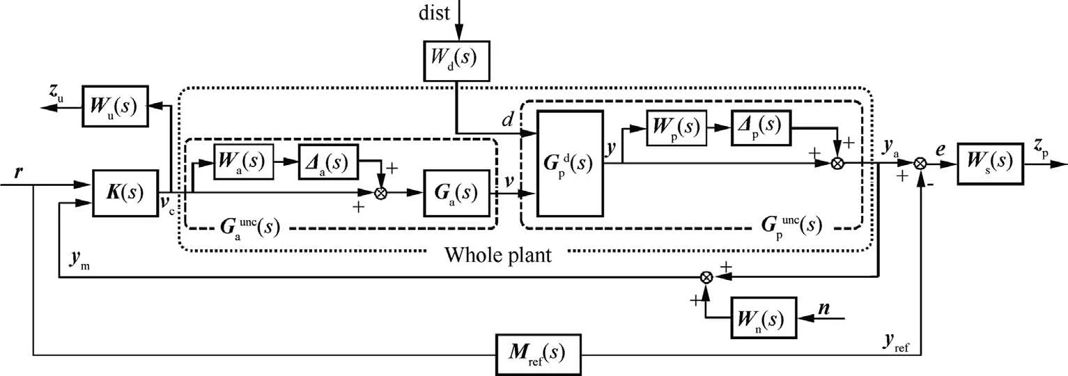
Fig.9 Block diagram of μ-synthesis design.

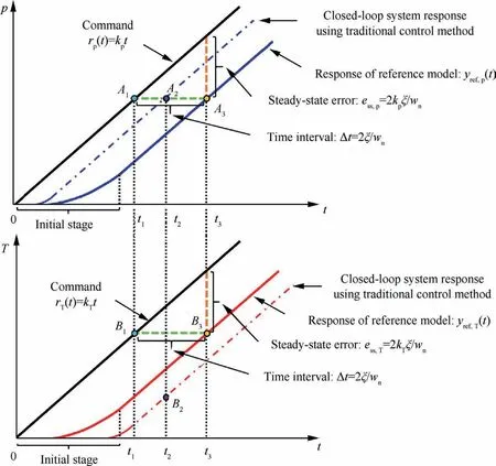
Fig.10 Schematic of ramp responses for pressure and temperature (kp and kT are any constants).

To ensure that the response of the closed-loop system can track the reference signal well, the performance weighting function Ws(s) has a large weighting over the low frequency range (see Fig.11(a)).Conversely, the control weighting function Wu(s) is small at low frequency.Then, the weight increases to the maximum at high frequency (see Fig.11(b)).This can exploit the full potential of the actuator and limit the magnitude of control actions.The performance weighting function and control weighting function are chosen as

3.3.μ-Synthesis design

For simplicity, the Laplace operator symbol s of the transfer function is sometimes ignored.The interconnected system shown in Fig.9 can be rearranged to fit the standard framework (see Fig.12).In Fig.12, the diagonal block Δ is structural uncertainty, expressed as

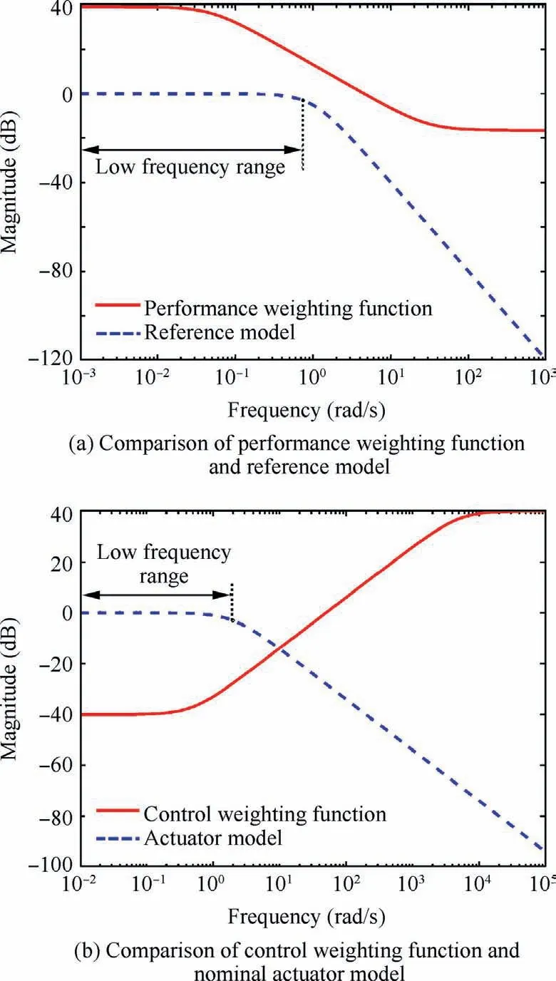
Fig.11 Magnitude responses of transfer functions.

μ-Synthesis is an effective method to deal with structural uncertainty.Its goal is to find a stabilizing controller K to minimize the peak value μΔ-（∙） of the closed-loop transfer function M.37This can be formulated as

Fig.12 Standard framework:Δ -P-K structure.

where M=FL（P，K）,and ˉΔ=diag[Δ，Δf],as shown in Fig.13(a).FL(∙,∙) represents the lower linear fractional transformation.Δfis a fictitious uncertainty block, which satisfies‖Δf‖∞≤1.17The structured singular value μΔ-（M ） is defined by

where σ-（∙） represents the largest singular value.det（∙） denotes the determinant.

Although the structured singular value μΔ-（∙）cannot be calculated exactly,D-K iteration is an efficient algorithm to solve the optimization problem shown in Eq.(36).38In this paper,utilizing the structure shown in Fig.12, D-K iteration is performed by MATLAB.39Then, the μ-controller (i.e., K(s)) can be computed.For implementation, the block diagram of ASTF’s control system is shown in Fig.14.

The closed-loop system shown in Fig.12 can be described by the standard M-Δ structure (see Fig.13(b)).According to the H∞norm bound of Δa1, Δa2, Δp1, and Δp2, we can know‖Δ‖∞≤1.Then, the necessary and sufficient condition for the robust stability of the closed-loop system is sup μΔ（M11）<1.Moreover, to guarantee the robust performance, we require sup μΔ-（M）<1.The thorough derivation and discussion of robust stability and robust performance can be found in Refs.17,38,40.Fig.15 presents the analysis results for the μ-controller.From Fig.15, we can see that the upper bounds of μΔ（M11） and μΔ-（M） are both less than 1 over the whole frequency range, which indicates that the designed controller can guarantee the robust stability and robust performance of the closed-loop system.

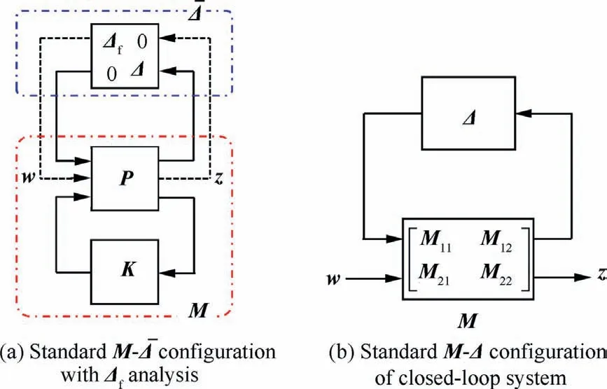
Fig.13 Standard configuration.

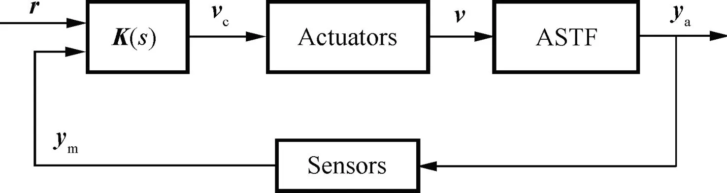
Fig.14 Block diagram of ASTF’s control system.

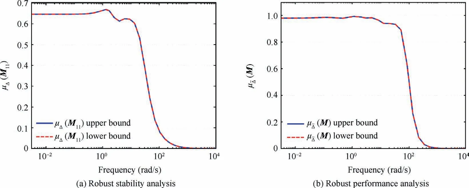
Fig.15 Bounds of structured singular value.

4.Simulation results

This section presents the simulation results.To avoid confusion, the designed μ-controller is called μmcontroller.The μmcontroller is compared with the multivariable PI controller,16integral-μ controller,10and LPV-based double integral-μ controller11to demonstrate the effectiveness of the proposed method.

4.1.Servo tracking performance

To test the servo tracking performance of the controllers,three cases of command signals are considered.In the first case, the command signal changes slowly within 5–45 s(called Stage A).In the second scenario, a step command is applied at 65 s(called Stage B).In the third case, the ramp command has a shorter duration of 5 s (called Stage C).

Figs.16 and 17 present the pressure and temperature responses of the airflow at the export, respectively.In Stage A, the double integral-μ controller has the minimum tracking error.Furthermore, considering the matching (see Remark 2)of temperature and pressure responses,the μmcontroller is also a good choice for ASTF.In Stage B, the responses of the closed-loop system with the μmcontroller can still track reference signals well.For the pressure response,the overshoot and relative steady-state error are 2.2% and 0.5%, respectively.For the temperature response, the overshoot and relative steady-state error are 1.9% and 0.5%, respectively.However,there are some oscillations and large overshoot in the system responses when the PI controller, integral-μ controller, and double integral-μ controller are used.The discordant dynamic responses are more obvious in Stage C, where the pressure response is faster than the temperature response.But the μmcontroller not only decouples the system dynamics, but also realizes the coordinated control of the pressure and temperature.Moreover, the change of the valve opening shown in Fig.18 reveals that the control valves move quickly and smoothly by using the μmcontroller.

4.2.Disturbance rejection performance

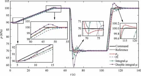
Fig.16 Comparison of pressure responses.

Fig.17 Comparison of temperature responses.

When the aircraft engine accelerates or decelerates, its intake airflow changes rapidly.This directly affects the pressure and temperature of the airflow at the export of ASTF.To analyze the disturbance rejection performance, we specify the flow change of the engine, as shown in Fig.19.The control objective is to keep the airflow pressure and temperature constant at 90 kPa and 280 K, respectively.The corresponding responses of the closed-loop system are shown in Figs.20 and 21.

The tracking errors of the closed-loop system with the μmcontroller are very small, which reveals that the μmcontroller can provide better disturbance rejection performance.Other controllers cannot quickly stabilize the system responses.This may affect the safety of ASTF.Moreover, in the presence of large disturbance (see 25–55 s in Figs.20 and 21), the relative errors of pressure and temperature responses of the system with μmcontroller are less than 3.2%and 0.23%,respectively.To further improve the control accuracy of the pressure, we can increase the gain coefficient kd(see Eq.(27)) in μsynthesis design.Thus, another simulation including three stages is performed, in which Stage D (i.e., 0–50 s) and Stage F (i.e., 70–110 s) are the disturbance tests at different steadystate points.Stage E(i.e.,50–70 s)is a step test.Fig.22 shows the flow change of the aircraft engine.

Fig.19 Flow change of aircraft engine.

Figs.23 and 24 present the impact of different kdvalues on the performance of the closed-loop system.As the gain coefficient kdincreases, the tracking performance (see Stage E) is basically unaltered,but the pressure fluctuation is greatly suppressed.For Stage D and Stage F,the maximum relative error of the pressure decreases by 0.62%, while the maximum relative error of the temperature increases by 0.1%.This can be acceptable.It should be noted that a large kdmay cause the peak values of μΔ（M11）and μΔ-（M）to rise(see Table 1).These peak values may exceed 1, implying that the robust stability margin and robust performance margin of the closed-loop system may decline.

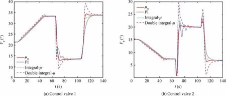
Fig.18 Change of valve opening.

Fig.20 Pressure responses in presence of disturbance.

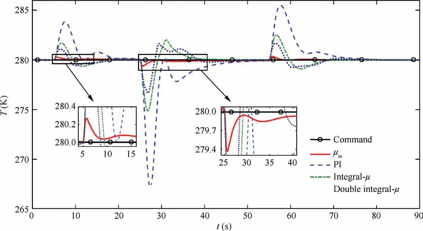
Fig.21 Temperature responses in presence of disturbance.

4.3.Robustness of closed-loop system

Actually,robustness with respect to uncertainties has been preliminarily verified in Sections 4.1 and 4.2.In this section, 100 sets of Monte Carlo simulations are performed to further evaluate the performance of the μmcontroller.For each Monte Carlo simulation,the key parameters(see Table 2)in the nonlinear model are randomly generated.

The Monte Carlo results are presented in Fig.26.Although the variation range of uncertain parameters exceeds the requirements in μ-synthesis design,the closed-loop system still achieves the desired performance.The pressure and temperature responses stably track reference signals, and the overshoots of both are less than 2.6%.Moreover, the rise time or settling time of each simulation is very consistent.From all the aforementioned simulations, the robust stability and robust performance of the closed-loop system subject to multi-source uncertainties are demonstrated.

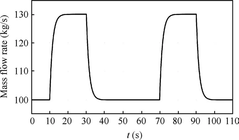
Fig.22 Flow change of aircraft engine in Stage D,Stage E,and Stage F.

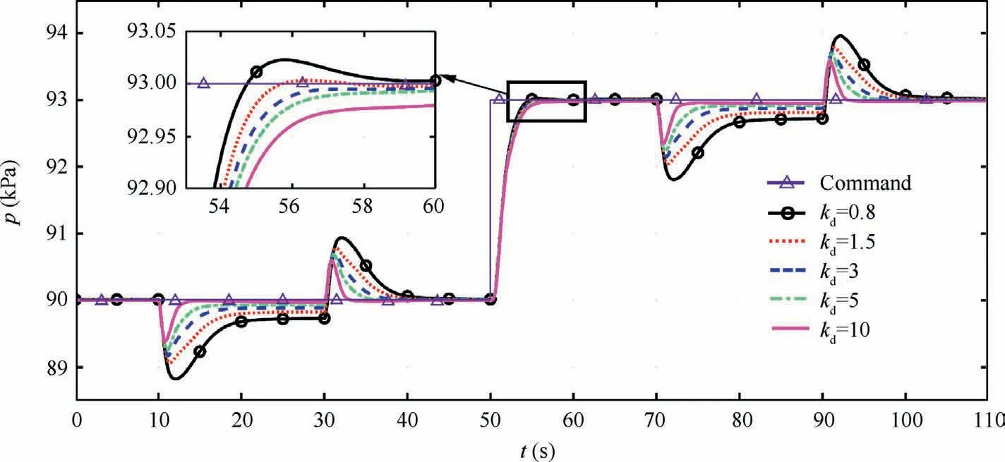
Fig.23 Pressure responses with different kd values.

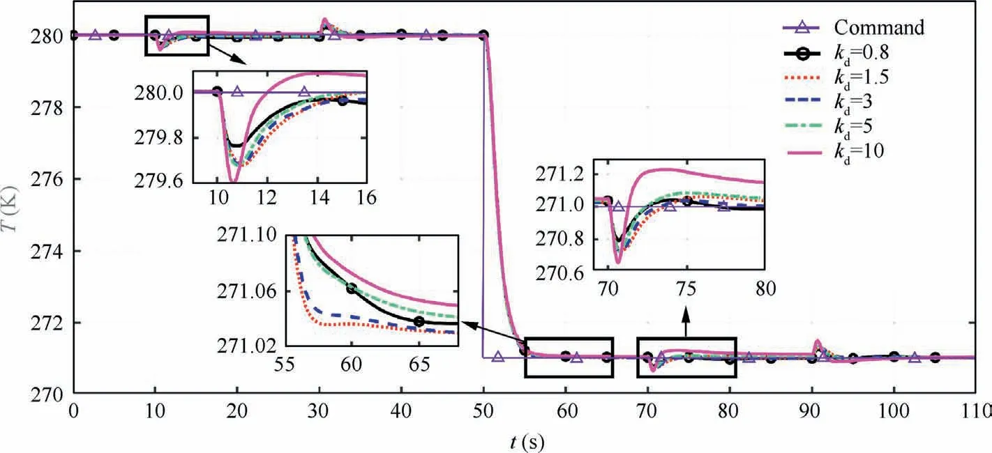
Fig.24 Temperature responses with different kd values.

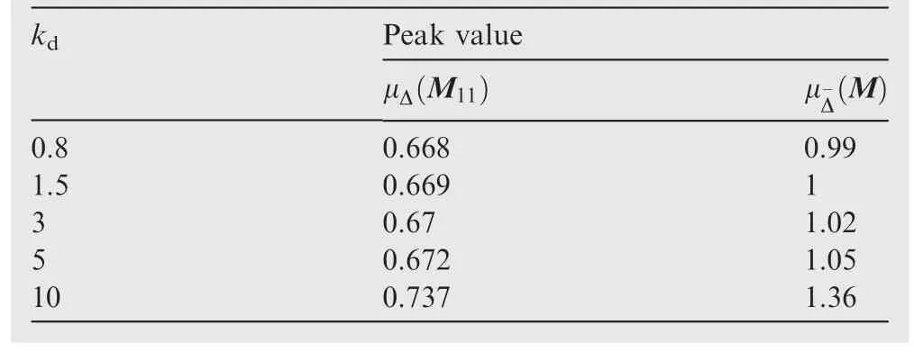
Table 1 Relationship between kd and peak value of structural singular value.

5.Discussion

As important characteristics of ASTF, dynamic coupling and multi-source uncertainties directly affect the performance of the closed-loop system.From the simulation results, it is difficult to guarantee the servo tracking performance and disturbance rejection performance by using the previous methods.The main reasons are summarized as follows:

Table 2 Variation range of uncertain parameters.

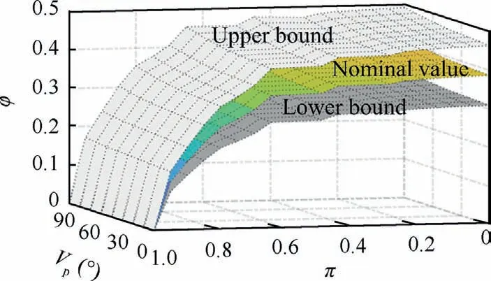
Fig.25 Variation range of flow coefficient.

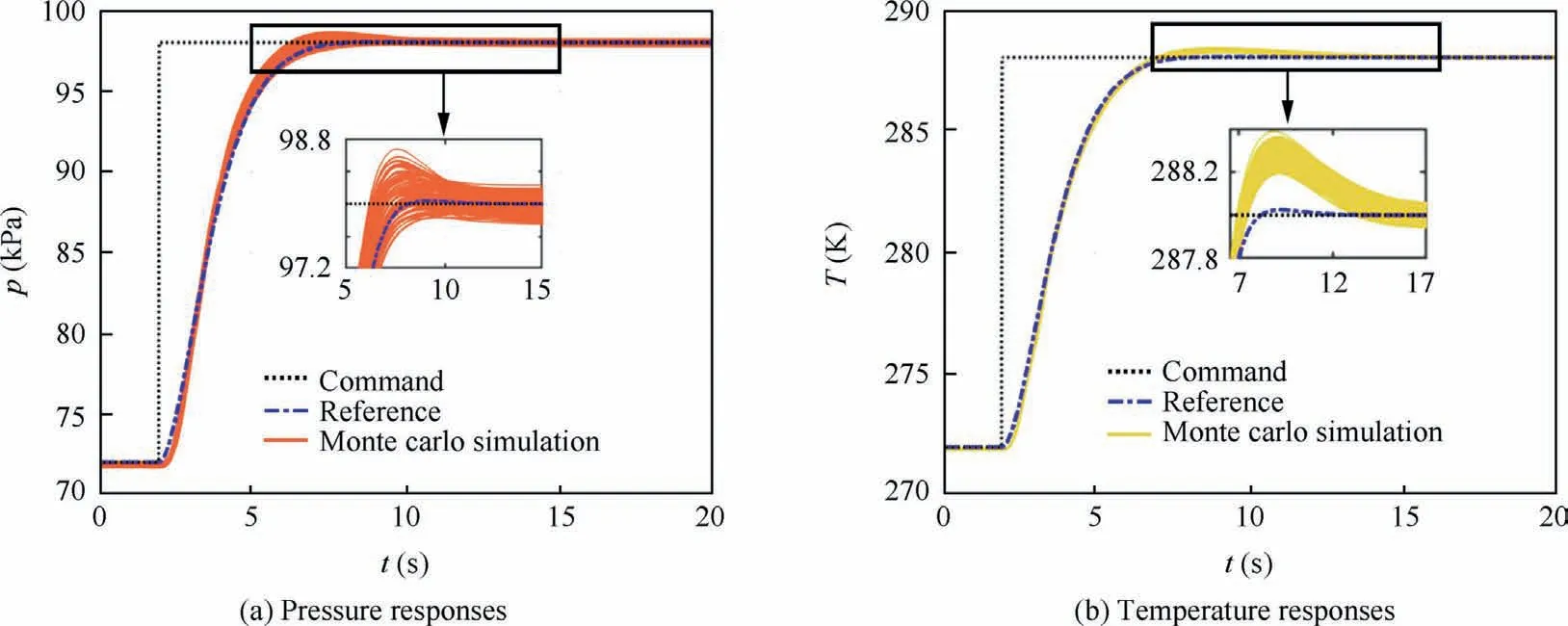
Fig.26 Monte Carlo simulation results.

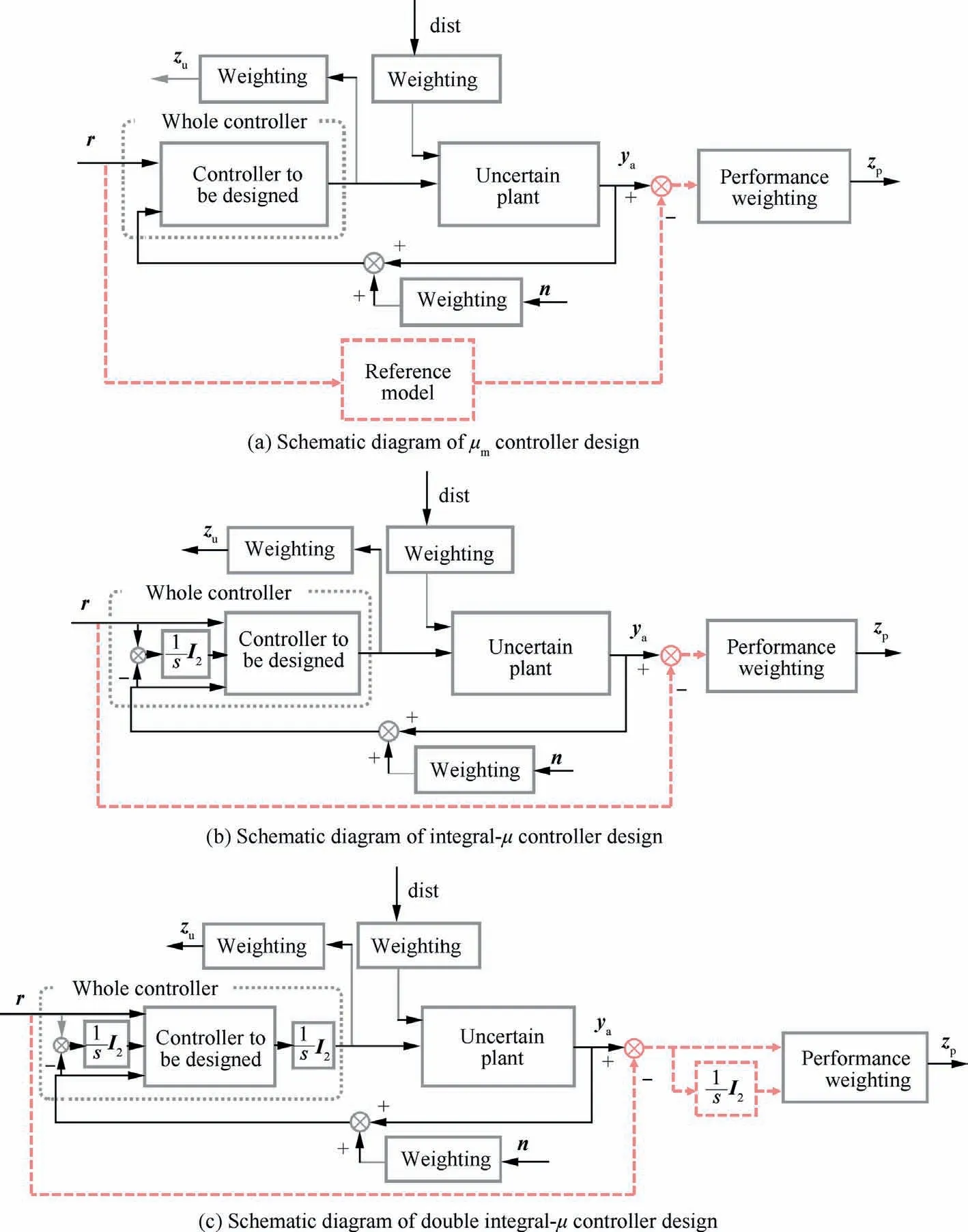
Fig.27 Comparison of various design frameworks.

(1) The multivariable PI controller is designed based on regional pole placement.However,it is difficult to determine a good pole region,nor to specify the relative position of the poles.Therefore, the dynamic coupling and multi-source uncertainties cannot be effectively handled.Furthermore, the matching of the pressure and temperature responses cannot be guaranteed.

(2) The design frameworks of the above μ controllers (i.e.,μm, integral-μ, and double integral-μ) are presented in Fig.27.To some extent, the integral-μ controller can be regarded as the μmcontroller whose reference model is an identity matrix in the design process.Then, the integral-μ controller enforces the system output to track the command signal, which causes larger control action and faster system response in the presence of rapid command(e.g., step command).This implies the occurrence of actuator saturation and large overshoot.For the design of double integral-μ controller, the integral of the tracking error is also weighted.This implies that the integral of the tracking error is expected to be small(i.e., close to 0).Therefore, overshoot and fluctuation are usually inevitable to eliminate the accumulation of the errors in the tracking process.

As shown in this paper,the proposed method has a superior performance, which benefits from the following aspects:

(1) The linear model of ASTF is improved to reduce the modeling error, which makes the controller less conservative.

(2) The parameter variations,modeling error in the low frequency range, unmodeled dynamics, and changes in the working point are simultaneously considered in the μsynthesis design, which ensures robust stability and robust performance.

(3) By using the diagonal reference model with desired performance in μ-synthesis design,the pressure and temperature dynamics are decoupled.

All of the above points are essential, and have not been thoroughly studied and discussed in previously published works.Recently, a dynamic event-triggered control method using a reference model was proposed, which can ensure the bounded tracking error.41Although it did not deal with various uncertainties,its idea can be introduced into the proposed method to further enhance the tracking performance.

6.Conclusions

This paper focuses on the high-precision control of the pressure and temperature of ASTF with dynamic coupling and multi-source uncertainties.The main conclusions are summarized as follows:

(1) By introducing the pressure ratio into the linear equation of the control valve, the modeling error of ASTF in the low frequency range is effectively reduced.On this basis, the uncertainties caused by modeling error,unmodeled dynamics, and changes in the working point can be clearly modeled.This is a key aspect of μ-synthesis design.

(2) The diagonal reference model in μ-synthesis can not only decouple the pressure and temperature dynamics,but also prescribe the desired dynamic performance.Compared with the multivariable PI controller,integral-μ controller, and double integral-μ controller,the proposed μ-controller has better servo tracking performance and disturbance rejection performance in the presence of rapid commands and large disturbance.

(3) The designed μ-controller can ensure the robust stability and robust performance of the closed-loop system in the presence of multi-source uncertainties.Moreover, the disturbance rejection performance can be improved as the gain of the disturbance weighting function increases,but the robust performance may decrease.

In the future,when the pressure and temperature of the air source are adjustable, the working envelope of ASTF will be further enlarged.In this case, it is necessary to further study the gain scheduling of μ-controllers while ensuring the control performance and robustness.

Declaration of Competing Interest

The authors declare that they have no known competing financial interests or personal relationships that could have appeared to influence the work reported in this paper.

Acknowledgements

The work was supported by the National Science and Technology Major Project, China (No.J2019-V-0010-0104), the Postdoctoral Science Foundation of China (No.2021M690289),the National Natural Science Foundation of China (No.52105138), and Zhejiang Provincial Natural Science Foundation of China (No.LQ23E060007).