Effect of internal defects on tensile strength in SLM additively-manufactured aluminum alloys by simulation

Xin SONG, Bowen FU, Xin CHEN, Jizhen ZHANG, Tong LIU,Chunpeng YANG, Yifn YE

a School of Mechanical Power Engineering, Harbin University of Science and Technology, Harbin 150080, China

b COMAC Beijing Aircraft Technology Research Institute, Beijing 102211, China

KEYWORDS

Abstract This research investigates the effect of internal defects on the tensile strength of Selective Laser Melting(SLM)additively-manufactured aluminum alloy(AlSi10Mg)test parts used for civil aircraft light weight design.A Finite Element Analysis(FEA)model containing internal defects was established by combining test data and the stress concentration factor comparison method.The effect of variation in the number,location and shape of defects on the finite element results was analyzed.Its results show that it is reasonable to use spherical defect modeling.The finite element modeling and analysis methods are also applied to the study of the effect of internal defects on tensile strength in additive manufacturing of other metallic materials.According to the FEA results of single defects at different scales, the formula for calculating the weakening degree of tensile strength applicable to the defective area of less than 15%was established.The result of the procedure is reliable and conservative.This research results can guide the selection of process parameters for the additive manufacturing of aluminum alloys.Further, the research results can promote the application of metal additive manufacturing in designing light-weight civil aircraft structures.

1.Introduction

Metal additive manufacturing technology has great potential for light weight design in civil aircraft structures.1However,Non-Destructive Testing (NDT) techniques reveal that different types of defects,including porosity,incomplete integration and cracks, inevitably appear inside the additivelymanufactured parts and that the appearance of defects is closely related to the selection of process parameters of additive manufacturing.2–5The presence of defects inevitably leads to local stress concentrations within the part, which weakens the mechanical properties of the part.Therefore, the control of the internal quality of parts and the establishment of technical standards are challenges that must be solved in the engineering application of metal additive manufacturing processes.Then quantifying the effect of defects on material properties is also an urgent topic of research.6,7Civilian structures are more concerned with the fatigue performance of the parts than the static performance.The effect of internal defects on fatigue performance is also more significant.However, there is currently no quantitative method for assessing the effect of defects on fatigue performance that can be used in engineering practice.7And tensile strength, as one of the critical mechanical properties of metal materials in engineering,is easily measured.It is widely used as a control index for product quality.In addition, the often used Hot Isostatic Pressing (HIP) posttreatment process can improve the fatigue properties of additively manufactured parts but will reduce the yield strength and tensile strength.Therefore, quantifying the effect of defects on the tensile strength of the material provides a reference for selecting additive manufacturing process parameters and determining internal quality assessment metrics.It has a direct contribution to the application of metal additive manufacturing process in designing light-weight civil aircraft structures.

At the same time, metal additive manufacturing is expensive,the cost of conducting this study through mechanical tests is high, and the test period is extended.Therefore, the quantitative analysis of the effect of defects on tensile strength in combination with elastic–plastic finite element simulation is an inexpensive and efficient research tool.8–12We need to establish a reasonable simplified geometric model containing defects, correctly assign material properties, boundary conditions to meet the actual situation as far as possible, select the appropriate cell properties, and set the proper mesh density,and choose a reasonable elastic–plastic and damage theory.13,14Verification tests according to uniaxial tensile test standards for metal materials are also a necessary task15,16to ensure the reliability of the analysis results of the elastic–plastic finite element simulation model.

There are many factors that affect the tensile strength of metal additives manufacturing parts, such as heat treatment method,test temperature,powder porosity,internal stress concentration, surface roughness, and material cross-sectional area.17,18However,the definition of tensile strength shows that the main effect is the reduction of the net cross-sectional area of the material due to the absence of internal material.19,20Therefore, this paper takes aluminum alloy additive manufacturing test parts as the research object and constructs an elastic–plastic FEA model with internal defects considered based on the test data of SLM additively-manufactured aluminum alloys (AlSi10Mg) test parts with and without prefabricated defects and proposes a method to improve the reliability of the model by correcting the number of finite element meshes with stress concentration coefficients to investigate the effect of variations in the type, scale, location and shape of internal flaws on the tensile strength at room temperature.

2.Finite element modeling of test parts with internal defects

2.1.Tensile strength test and defective NDT data

The aluminum alloy samples used in the test were prepared by Selective Laser Melting (SLM) process, including ten samples without prefabricated defects and five spherical samples with prefabricated defects with different diameters of 0.3, 0.4, 0.8,1.2, and 2.0 mm.The printing parameters are printing layer thickness 0.03 mm, scanning pitch 0.19 mm, laser power 370 W, scanning speed 1300 mm/s, annealing heat treatment after printing, temperature 300 ℃and holding time 2 h.The defect is located at the middle axis of the sample.The X, Z,and 45 in the sample number indicate the angle between loading direction and printing direction 0°, 90° and 45° respectively.All samples are made of the same batch of aluminum alloy powder material, machine, process parameters, and heat treatment method.One of the processed samples and its geometric dimensions are shown in Fig.1.

Before the test, the pre-defective samples were inspected non-destructively, using an YXLON FF35 high-resolution CT machine with 5 μm resolution for layered scanning.Because the metal powder inside the pre-set defect could not be excluded, when the defect diameter was small, its shape was non-regularly spherical.The boundary scanned was not very clear, the actual size of the defect was determined by the maximum identifiable boundary.The results of the fourview scanning are shown in Fig.2.The lower right figure shows the spatial defect location and coordinate system schematic, and the remaining three views are tomographic scans of the maximum defect size in three directions.When modeling the defect geometry in Finite Element Analysis (FEA) software, the actual dimensions obtained from the NDT scan and modeled as an ideal spherical shape were used to get a biased conservative analysis.The actual defect scales are shown in Table 1.

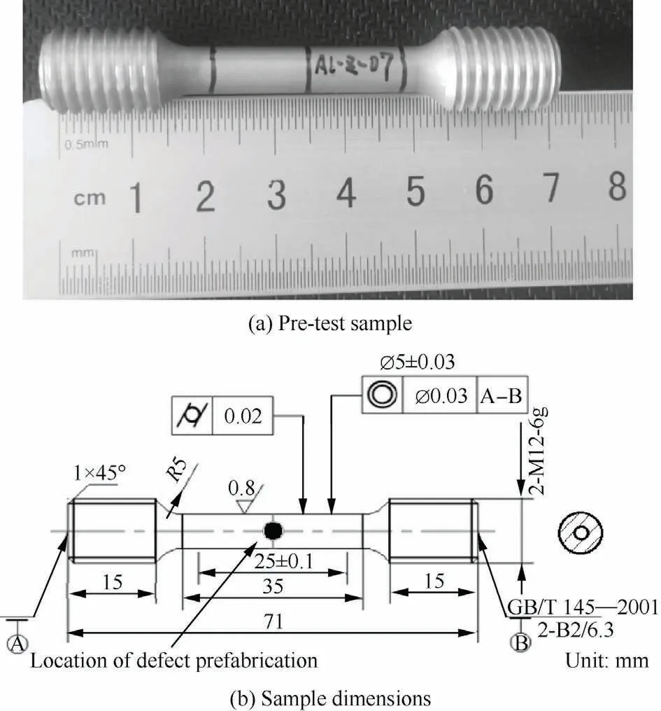
Fig.1 Additively-manufactured sample for tensile test.

Fig.2 Scanning electron micrograph of samples with prefabricated defects.

The tensile test of the sample refers to the Chinese national standard GB/T 228,using the calibrated WDW electronic universal testing machine for the test,as shown in Fig.3.According to the standard, the tensile strength is calculated as

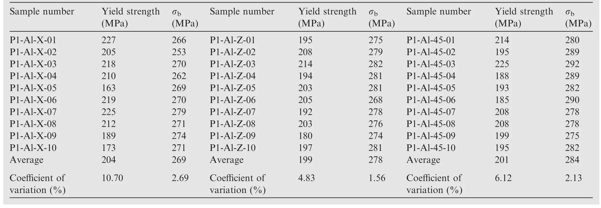
where Fmaxis the ultimate tensile load; A0is the initial crosssectional area of the sample.The samples after the test are shown in Fig.4, and the test results are shown in Table 2.

According to the test data in Table 2,the average values in the X-direction and 45°direction differ by–3.24%and 2.16%,respectively, compared to the Z-direction test data.Less errorin the data, it is reasonable to assume that the material is isotropic in the finite element analysis.The Z-directional test data is also used as the baseline data for modeling and calibration.The fracture test data for the Z-direction without pre-set defects and prefabricated defect test pieces are shown in Table 3.

Type Defect diameter (mm)Theoretical 0.3 0.4 0.8 1.2 2.0 Actual 0.60 0.78 1.16 1.66 2.50

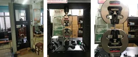
Fig.3 WDW universal testing machine and sample clamping.

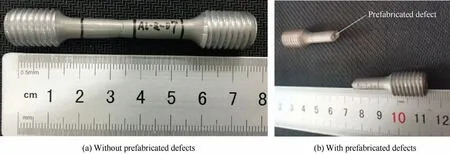
Fig.4 Post-test samples.

2.2.Establishment of elastic–plastic FEA model for sample without prefabricated defects

ABAQUS finite element software has potent functions in material nonlinear analysis, especially in material elastic–plastic analysis.It can judge each deformation stage of the material based on the input elastoplastic parameter values and present the material deformation behavior in the form of unit deformation.Combined with the defined damage parameters, the fracture of the model is achieved by deleting cells when the plastic deformation reaches the set damage parameters.That is, the finite element analysis process simulates the plastic deformation and fracture process of the samples.

2.2.1.Geometric modeling

The geometric model should be built according to the geometry shown in Fig.1(b) to ensure the accuracy of the FEA results.However, the standard sample clamping method has a negligible effect on the test results.19Therefore, when building the finite element model, the threads are simplified with cylinders to improve the FEA efficiency.

In addition, it can be found from the scan results of Fig.2 that there are still some small-scale defects inside the rest of the test piece,in addition to the preset defects.It means that there are similar small defects inside the test piece without prefabricated defects.Ref.20 concluded that these small defects have little effect on the tensile strength.In order to reduce the com-plexity of finite element modeling, it can be disregarded for now.And the effects produced by these small defects are analyzed in detail after the preliminary finite element analysis results are obtained.

Sample number Yield strength(MPa)σb σb σb(MPa)P1-Al-X-01 227 266 P1-Al-Z-01 195 275 P1-Al-45-01 214 280 P1-Al-X-02 205 253 P1-Al-Z-02 208 279 P1-Al-45-02 195 289 P1-Al-X-03 218 270 P1-Al-Z-03 214 282 P1-Al-45-03 225 292 P1-Al-X-04 210 262 P1-Al-Z-04 194 281 P1-Al-45-04 188 289 P1-Al-X-05 163 269 P1-Al-Z-05 203 281 P1-Al-45-05 193 282 P1-Al-X-06 219 270 P1-Al-Z-06 205 268 P1-Al-45-06 185 290 P1-Al-X-07 225 279 P1-Al-Z-07 192 278 P1-Al-45-07 208 278 P1-Al-X-08 212 271 P1-Al-Z-08 203 276 P1-Al-45-08 208 278 P1-Al-X-09 189 274 P1-Al-Z-09 180 274 P1-Al-45-09 199 275 P1-Al-X-10 173 271 P1-Al-Z-10 197 281 P1-Al-45-10 195 282 Average 204 269 Average 199 278 Average 201 284 Coefficient of variation (%)(MPa)Sample number Yield strength(MPa)(MPa)Sample number Yield strength(MPa)10.70 2.69 Coefficient of variation (%)4.83 1.56 Coefficient of variation (%)6.12 2.13

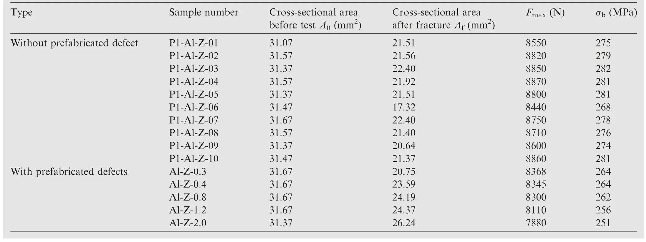
Type Sample number Cross-sectional area before test A0 (mm2)Cross-sectional area after fracture Af (mm2)Fmax (N) σb (MPa)Without prefabricated defect P1-Al-Z-01 31.07 21.51 8550 275 P1-Al-Z-02 31.57 21.56 8820 279 P1-Al-Z-03 31.37 22.40 8850 282 P1-Al-Z-04 31.57 21.92 8870 281 P1-Al-Z-05 31.37 21.51 8800 281 P1-Al-Z-06 31.47 17.32 8440 268 P1-Al-Z-07 31.67 22.40 8750 278 P1-Al-Z-08 31.57 21.40 8710 276 P1-Al-Z-09 31.37 20.64 8600 274 P1-Al-Z-10 31.47 21.37 8860 281 With prefabricated defects Al-Z-0.3 31.67 20.75 8368 264 Al-Z-0.4 31.67 23.59 8345 264 Al-Z-0.8 31.67 24.19 8300 262 Al-Z-1.2 31.67 24.37 8110 256 Al-Z-2.0 31.37 26.24 7880 251

2.2.2.Determination of elastic–plastic and damage parameters

Due to the presence of internal defects and variations in additive manufacturing parameters that can have an impact on the elastic properties of the material.Therefore,the material property parameters determined from the manual or literature must also be verified and adjusted in conjunction with the experimental results to make the simulated material behavior more closely match the tests.

The elastic parameters in the elastic–plastic finite element analysis are mainly the tensile modulus E, Poisson’s ratio μ,and the density ρ has negligible effect on the finite element analysis results.The damage mechanics concept was applied in Ref.21 to establish the relationship equation between the pore volume fraction (φ) and the measured tensile modulus(Et) and the tensile modulus of an ideal material (E):

In Refs.22,23 which studying comparative analysis of porosity measurement methods for additive manufacturing,the maximum porosity of specimens prepared with different process parameters was less than 50%.From Eq.(2), it is obtained that Etwill not vary by more than 50%.

Based on experimental data and as determined in the literature, the elastic parameters can be obtained from the experimental data as well as from the test data and Ref.16, with tensile modulus E = 70 GPa, Poisson’s ratio μ = 0.34 and density ρ = 2.6 g/cm3.Analyze the effect of variation of E and μ on FEA results.The results of the analysis are shown in Table 4.

It can be seen that the variation of Poisson’s ratio is negligible for the finite element results.As the value of tensile modulus decreases, its tensile strength decreases, but the effect is not significant.Therefore, without considering the effect of defects on their tensile modulus, the results can also meet the engineering applications.

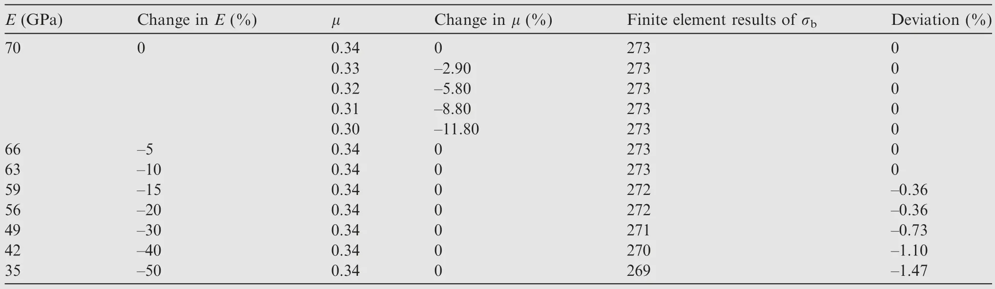
E (GPa) Change in E (%) μ Change in μ (%) Finite element results of σb Deviation (%)70 0 0.34 0 273 0 0.33 –2.90 273 0 0.32 –5.80 273 0 0.31 –8.80 273 0 0.30 –11.80 273 0 66 –5 0.34 0 273 0 63 –10 0.34 0 273 0 59 –15 0.34 0 272 –0.36 56 –20 0.34 0 272 –0.36 49 –30 0.34 0 271 –0.73 42 –40 0.34 0 270 –1.10 35 –50 0.34 0 269 –1.47

The von Mises yielding criterion was used for the plasticity analysis,the hardening plasticity index is isotropic because the tensile test is relatively simple and the isotropic assumption was made above.The plastic parameters are mainly real stress σt, real strain εtand equivalent plastic strain εpl.Since the test records the data of nominal stress σεand nominal strain εε,the relationship between the parameters can be converted by the mechanical Eqs.(3)–(5):

The data acquisition interval of the tester is 0.05 s, and the total number of stress–strain data pairs is 3442.The import function of the finite element software can be used to input the actual stress and plastic strain into the plasticity parameter table to build the material plasticity model.

The kinetic display algorithm was selected when performing fracture simulations.Among the seven ductile metal damage models in ABAQUS, Forming Limit Diagram (FLD),Forming Limit Stress Diagram (FLSD), Marciniak-Kuczynski (M-K) and Muschenborn-Sonne Forming Limit Diagram (MSFLD) are suitable for analyzing the damage to thin metal sheets.Shear damage was then applied to the shear test.Although Johnson-Cook damage is more comprehensive in its considerations, it is more suitable for high-temperature tests because of the temperature and melting point changes involved.Since this test is a uniaxial tensile test at room temperature,which does not include temperature change,and it is a standard sample in the form of a bar,the ductile damage was chosen as the damage model for the finite element.

The fracture strain can be calculated by

where A0is the initial cross-sectional area; Afis the crosssectional area after fracture.

In the ductile damage model, the damage parameters required are the fracture strain εf, plastic strain ratio and the stress triaxiality σav.εfcan be calculated from the data of P1-Al-Z-07 in Table 3 using Eq.(6).The plastic strain ratio,also called the thick anisotropy coefficient,is an essential index for evaluating the performance of the sample.It reflects the difference between the strain capacity in the plane direction and the thickness direction of the sheet.The coefficient exhibits anisotropy when it is greater than 1 and isotropy when it equals 1.Since the material used in the test was a bar sample,and the material was considered isotropic in the analysis, the strain ratio was 1.σavis defined as the ratio of hydrostatic stress to Mises stress.It can be directly selected by the stress triaxiality values of the standard test in Ref.24.

The damage displacement in the damage evolution can control the displacement value of the finite element output,so the parameter needs to be adjusted after the other parameters are determined.As a result,the displacement output from the calculation is close to the displacement value obtained from the test.The final results of the damage parameters are shown in Table 5.

2.2.3.Setting boundary conditions and meshing

The lower clamping end of the sample was fixed, and the reference point was set and coupled to the outer surface of the upper clamping end in order to apply the load and the output curve to compare the test data.A tensile load was applied to the reference point in the direction of the axis.The C3D8R cell type is suitable for elastic–plastic analysis.In addition, mesh density is an important factor affecting the accuracy of elastic–plastic finite element results.However,there is no quantitative method to calibrate the grid density.Only the lower threshold value is guaranteed, and there is no upper limit on the number of grids required.Although the denser the mesh,the higher the analytical accuracy,the two are not linearly correlated.25Too thick a grid is ineffective in improving the accuracy, and reducing the computational efficiency.

Experimental data can be used for FEA models without prefabricated defects to determine the appropriate mesh density.First, the damage displacement was set to a small value,using the default mesh size with the fracture displacementvalue given by the testing machine.Next, displacementcontrolled loading was performed, and the FEA results of the ultimate tensile load value and total displacement were obtained according to the force–displacement graph at the reference point.Then,the maximum tensile load output from the finite element was made to approximate the value given by the test machine by continuously encrypting the mesh.Eventually,the error with the test was minimized when the grid size was adjusted to 1 mm.The outcome of the FEA simulation is shown in Fig.5.The elastic–plastic FEA model is shown in Fig.6.

Fracture strain Disruption of displacement 0.37 1 0.33 0.3 Plastic strain ratio Stress triaxiality

2.3.Building an FEA model with defects

In an FEA model without prefabricated defects, internal defects can be created using the material removal function in the ABAQUS.Since the shape of defects inside additively manufactured metal parts is usually irregular,regular processing is required for modeling.Pore defects can be regularized to spherical or ellipsoidal shape.26

Unfused defect can generally reach the millimeter level in size and affects the tensile strength of the part to a much deeper degree.27The shape of such defects is usually manifested as flakes or cracks.28,29Regularization is carried out in the shape of a hexahedron while ensuring the same maximum crosssectional area of the defect.Among them, the defects caused by the under-filling of molten metal are treated with lamellar hexahedral metal, as shown in Fig.7.30Crack defects caused by poor lap of the sweep line are treated with rod-shaped hexahedra.The schematic diagram of the finite element model with defects is shown in Fig.8.

In addition, for models containing internal defects, the requirements for mesh density are higher when performing elasticity analysis due to the large stress concentration at the defect boundary.A method is proposed to debug the mesh using the stress concentration factor KT.This method determines the number and scale of grids more efficiently and accurately.KTis the ratio of the maximum local elastic stress σmaxto the nominal stress σe.The theoretical value of the simple structural details in the online elastic state can be obtained precisely.The stress concentration coefficient query manual25is an academic manual that has been verified and widely used in engineering practice,from which we can obtain the theoretical values.With the development of computer technology and the improvement of finite element theory,the stress concentration coefficients obtained by numerical calculation methods can be combined with finite elements to accurately approximate the actual situation.

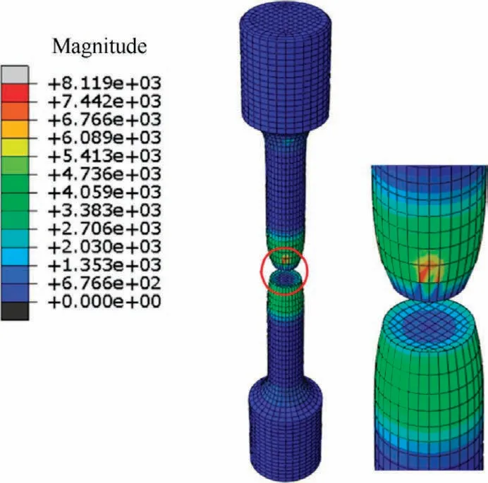
Fig.5 Outcome of FEA simulation.

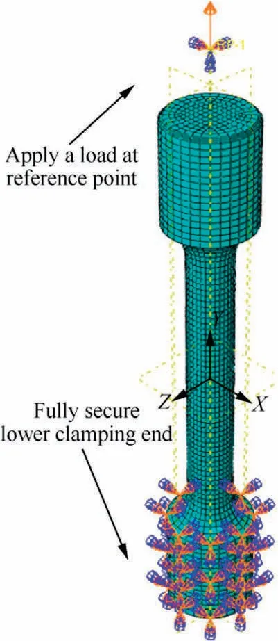
Fig.6 Simulation constraints.

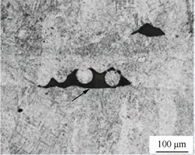
Fig.7 Unfused defects.30

Fig.8 Regularized defect model.

A physical model that is more compatible with the experimental model can be built according to the model in the stress concentration factor manual.The model was given a load of 5000 N and the same elastic material parameters as the test to build a finite element model in the elastic range for analysis.The nominal stress was calculated as 177 MPa.Finally, the grid cell property C3D20 was selected, suitable for calculating the stress concentration.The stress concentration coefficients at different grid densities were calculated by continuously encrypting the grid to compare with the theoretical values.Finally,the appropriate number of grids was determined.Calculations were performed on a 0.4 mm defect scale, and the theoretical stress concentration factor was queried in the root manual.

According to this method, it can be seen that the actual stress concentration coefficient deviates the least from the theoretical stress concentration coefficient value when the grid size is 0.8 mm, and the number of grids is about 8000, as shown in Table 6.The accuracy and computational efficiency of the FEA are optimal at this point.

3.Simulation analysis of effect of defects on tensile strength

3.1.Finite element model accuracy verification results

From Table 7, it can be seen that the defects of less than 100 μm in size are neglected in the finite element modeling.Therefore, when the defect scale is small (diameter less than 2.5 mm), the tensile strength obtained from the finite element simulation of the sample is greater than the test data,and using it as the design value will give non-conservative results.Since the deviation of the values does not exceed 4%,it confirms that the FEA model with internal defects is reasonable and reliable.Thus, it can be used for simulation test analysis in different defect cases.

3.2.Effects of defects on tensile strength of material

The FEA results show that, the presence of defects leads to a reduction in net cross-sectional area and localized stress concentrations that affect the material’s tensile strength.The scale of a single defect and the combined effect of multiple defects can reduce the net cross-sectional area.Besides, the shape and location of the defect will cause the local stress concentration of different degrees.The defect’s shape also affects how the microscopic particles at the edge of the defect are arranged,thus affecting the results judged by net cross-sectional area and stress concentration alone.The effect of defects on the tensile strength of the material is analyzed from the following three aspects.

3.2.1.Effect of defect scale on tensile strength

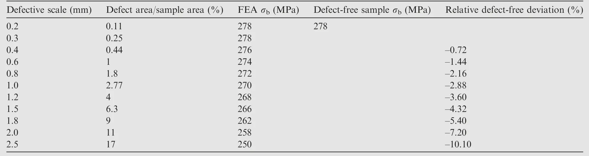
When the process parameters of additive manufacturing are not chosen properly,large-scale porosity may occur.The accuracy of current ultrasonic monitoring equipment can detect defects as small as 200–660 μm.28Therefore, a series of finite element models with different scales of defects have been developed to analyze the effect of defect scale on tensile strength when only a single defect is considered.The results of the analysis are shown in Table 8.

The percentage of the cross-sectional area(Ad)of the defect relative to the nominal area (A0) of the specimen is the variable.Adis defined as the projected area of the cross-section at the largest scale of the defect.

Using the data in Table 8, the effect of defect scale on tensile strength can be fitted with a polynomial given by

where y is the degree of weakening of the tensile strength, %;x = Ad/A0.Fitting correlation R2= 0.968.

To obtain more accurate and conservative FEA results, a correction to Eq.(7)is required,mainly considering the following aspects.

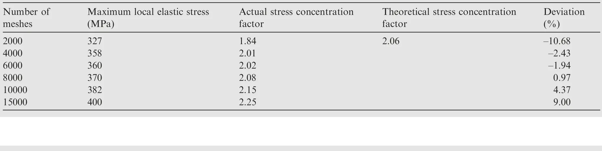
Number of meshes Deviation(%)2000 327 1.84 2.06 –10.68 4000 358 2.01 –2.43 6000 360 2.02 –1.94 8000 370 2.08 0.97 10000 382 2.15 4.37 15000 400 2.25 9.00 Maximum local elastic stress(MPa)Actual stress concentration factor Theoretical stress concentration factor

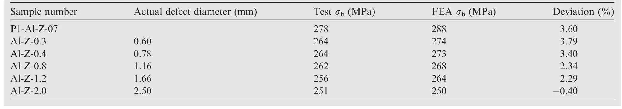
Sample number Actual defect diameter (mm) Test σb (MPa) FEA σb (MPa) Deviation (%)P1-Al-Z-07 278 288 3.60 Al-Z-0.3 0.60 264 274 3.79 Al-Z-0.4 0.78 264 273 3.40 Al-Z-0.8 1.16 262 268 2.34 Al-Z-1.2 1.66 256 264 2.29 Al-Z-2.0 2.50 251 250 -0.40

?

(1) Although isotropic assumptions were used in the finite element analysis, it can be seen from Table 2 that there are still differences in the experimental data for different printing directions, with negative deviation leading to non-conservative finite element results with a deviation of 3.24%.

(2) From Table 4, it can be seen that the deviations due to material elasticity changes lead to biased conservative finite element results with a maximum deviation of 1.91%.

(3) The bias caused by the setting of the mesh density leads to biased conservative finite element results with a bias of 0.97%.

(4) The scale of internal porosity defects produced by SLM process is mainly concentrated in 20–30 μm.A small number of defects on a larger scale are not more than 100 μm, and all are Gaussian distributed centered at 0.9.31Assume that the scale of these defects was upper 100 μm.Then the Ad/A0of single defect is 0.027%.According to Table 8, it can be seen that the effect of defects can be neglected when Ad/A0< 0.44%.Based on the NDT results in Fig.2, it is reasonable to disregard small defects in the modeling.

Considering the effects of material anisotropy,variations in E,variations in mesh density,and instability in the number of small defects,a combined impact factor KZis added to Eq.(7)to obtain a more conservative result, as

Based on the experimental data and analysis results,KZ= 1.18 was initially set.

The simulation analysis of a single defect is a simplified treatment of an ideal situation.In practice, there is usually more than one defect in the same section.So,when calculating the total area of defects,it is not just a simple accumulation of all defects but also needs to consider the interaction between two adjacent defects.When two defects are close, the defects can be equated using the method described in Ref.32.As shown in Fig.9, when the defect edge e is smaller than the diameter d2of the smaller defect,the two defects will be treated as being merged.The area of the defect after equivalence is the area included in the dotted line.At the same time, the defects of different cross-sections with close spacing also need the same equivalent treatment.

This subsection takes two adjacent defects with a scale of 0.4 mm.Defects were set in the same section and different sections in two distributions within the distance section.Then defect equivalence analysis was performed.Fig.10 shows a schematic diagram of two defects in different sections and equivalent in the same section.

Ad/A0will be changed as a percentage of the nominal area of the sample because the equivalent will become a larger scale defect.The effect of defects on tensile strength will also change.The FEA results are shown in Table 9.

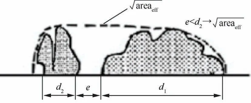
Fig.9 Defect equivalence method.

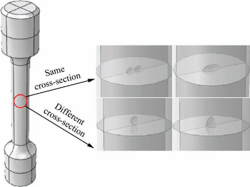
Fig.10 Different sections and same section defects equivalent before and after effect.

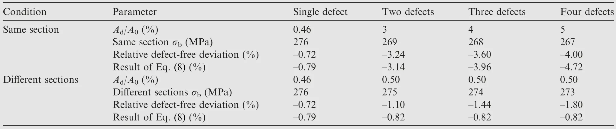
Condition Parameter Single defect Two defects Three defects Four defects Same section Ad/A0 (%) 0.46 3 4 5 Same section σb (MPa) 276 269 268 267 Relative defect-free deviation (%) –0.72 –3.24 –3.60 –4.00 Result of Eq.(8) (%) –0.79 –3.14 –3.96 –4.72 Different sections Ad/A0 (%) 0.46 0.50 0.50 0.50 Different sections σb (MPa) 276 275 274 273 Relative defect-free deviation (%) –0.72 –1.10 –1.44 –1.80 Result of Eq.(8) (%) –0.79 –0.82 –0.82 –0.82

Defective scale (mm) Different defects amount in same cross-sectional area with same Ad/A0 Ad/A0 (%) σb (MPa) Deviation (%)0.4 1 0.44 276 0.40 4 0.44 277 8 0.44 277 0.6 1 1.00 274 4 1.00 274 8 1.00 274 0.8 1 1.80 272 4 1.80 272 8 1.80 272 1.0 1 2.78 270 4 2.78 270 8 2.78 270

From the analysis results, it can be seen that the different morphologies of the defect after equivalence leads to different degrees of material loss in its dangerous cross-section.That is,the net cross-sectional area within the fracture cross-section is different.Within the same cross-sectional area,the greater the number of adjacent defects in the equivalent treatment, the greater the effect on the material’s tensile strength.The equivalent treatment of defects in different cross-sections has little effect on the material’s tensile strength because the net crosssectional area remains the same as the number of defects increases.Regardless of the adjacent defects within the same section or within different sections, the deviation between the FEA and the effect of defects on tensile strength calculated using Eq.(8), when treated equivalently, is less than 1% in both cases.This demonstrates that Eq.(8) applies equally to the case of adjacent defects that have been equivalently treated.

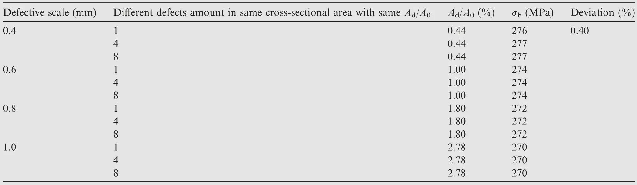
When e > d2, the defects in the same section can be regarded as independent of each other.The total defect area is the cross-sectional accumulation of multiple defects.The tensile strength of a single defect with the same or close to Ad/A0as the base to build finite element models with a different number of defects.The results of the FEA are shown in Table 10.From the analysis results, single defect and multiple defects of the same or close to Ad/A0in both cases, the deviation of the analytical results of the effect of defects on tensile strength is negligible.This means that Eq.(8) is equally applicable to the case of multiple defects with large spacing.

3.2.2.Effect of defect location on tensile strength

By using Eq.(9)given in the stress concentration handbook,33we can see that the stress concentration factor KTis influenced by the distance from the center of the defect to the closer edge of the specimen c,the distance of the defect from the more distant edge e′and the diameter of the defect d.As c/e′decreases and d/c increases,the stress concentration factor caused by the defect increases, which leads to a decrease in the σb.

Fig.11 Defect locations and scale adjustment.

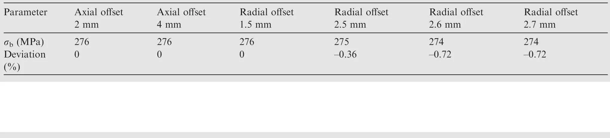
Parameter Axial offset 2 mm Radial offset 2.7 mm σb (MPa) 276 276 276 275 274 274 Deviation(%)Axial offset 4 mm Radial offset 1.5 mm Radial offset 2.5 mm Radial offset 2.6 mm 0 0 0–0.36 –0.72 –0.72

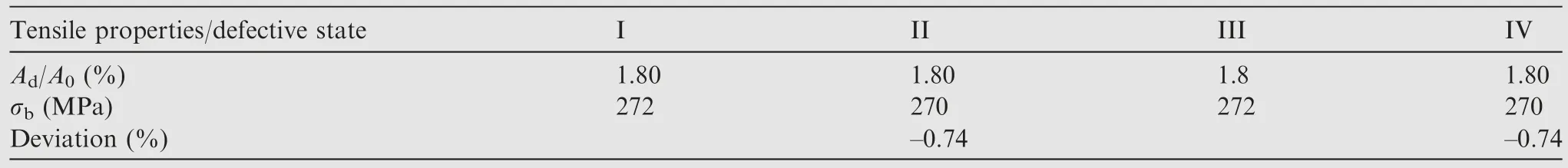
Tensile properties/defective state I II III IV Ad/A0 (%) 1.80 1.80 1.8 1.80 σb (MPa) 272 270 272 270 Deviation (%) –0.74 –0.74

For a single defect,analyze the variation of the defect position along the axial and radial directions,respectively.For the case of multiple defects(Fig.9,e>d2),the change in position of multiple defects within the same section was analyzed.The finite element analysis model for the change of defect position is shown in Fig.11.Taking the defect scale of 0.4 mm as an example, the other parameters to control the defect are the same.Based on the result of a single defect with the center of the defect in the center of the sample (σb= 276 MPa).The results of finite element analysis are shown in Tables 11 and 12.From the results, it can be seen that the change of defect location has negligible effect on the σb.

3.2.3.Effect of defect shape on tensile strength

Due to the variability of additive manufacturing process and a large number of process parameters, the causes of defect formation are different, resulting in different shapes of defects.Most exhibit a spherical or ellipsoidal shape.For ellipsoidal defects, the degree of stress concentration generated at the edges of the section will vary due to ellipsoidal shapes with different long and short axes.Therefore, its long and short axis ratio is changed by taking 0.4 mm defect volume as the base,which are 2.5, 2.0, 1.5, 1.0, 0.67, 0.5, 0.4, respectively.The shape of the formed defect is shown in Fig.12.

Unfused and cracked defects are characterized by a large defect scale, shape close to the hexahedron, the arrangement between defects more regular.34Therefore, cubic and specially shaped hexahedral defects were created separately to analyze the effect of defect shape on σb.Among them, hexahedral defects include lamellar hexahedra and rod-shaped hexahedra were used to simulate unfused defects as well as cracked defects, respectively.

The analyzed data are shown in Table 13.The effect of the change in the shape of the ellipsoidal defect is mainly reflected in the change in Ad/A0.It is reasonable to use spherical defect modeling.The calculated results of Eq.(8) do not deviate much from the results of the finite element analysis of ellipsoidal defects of different shapes.From the results in Table 14,it can be seen that for different shapes of hexahedral defects,when Ad/A0is the same (Ad/A0= 14%), the effect of defects on the same.That is, the defect shape change has no effect on finite element results.In addition, due to the regulated atomic arrangement of the grains at the edges of the hexahedral defects, forming stable boundaries that are difficult to move.The defect edges of the hexahedra did not show atomic dislocations before and after stretching.At the edges of spherical defects,atoms are more prone to dislocations,35leading toa greater impact of spherical defects on the σb.In the case of Ad/A0< 15%, a conservative result can be obtained using Eq.(8) to calculate the effect of defects on σb.

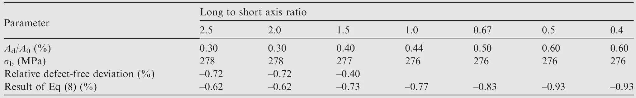
Long to short axis ratio 2.5 2.0 1.5 1.0 0.67 0.5 0.4 Ad/A0 (%) 0.30 0.30 0.40 0.44 0.50 0.60 0.60 σb (MPa) 278 278 277 276 276 276 276 Relative defect-free deviation (%) –0.72 –0.72 –0.40 Result of Eq (8) (%) –0.62 –0.62 –0.73 –0.77 –0.83 –0.93 –0.93 Parameter

Type Ad/A0 (%) σb (MPa) Relative defect-free deviation (%) Result of Eq.(8) (%)Cube defects 0.88 277 –0.04 –1.20 2.26 276 –0.72 –2.50 3.5 275 –1.10 –3.56 8 265 –4.70 –6.60 14 257 –7.55 –8.70 Flaky unfused defects 5 273 –1.80 –4.72 9 264 –5.04 –7.12 14 257 –7.55 –8.70 Rod crack defect 5 273 –1.80 –4.72 9 264 –5.04 –7.12 14 257 –7.55 –8.70

4.Conclusions

(1) Net cross-sectional area is the main factor affecting the material’s tensile strength.The defective areas accounted for no more than 15%combined with a small amount of test data to reasonably adjust the value of the comprehensive impact factor KZ.It is reliable and conservative to estimate the effect of defects on tensile strength using the proposed equation.The selection of quality standards and process parameters for additively manufactured products of AlSi10Mg aluminum alloys can be guided.

(2) The finite element modeling and analysis method using spherical defects is also applicable to studying the effect of internal defects on tensile strength in additive manufacturing of other metallic materials.The research results can promote the application of metal additive manufacturing process in designing civil aircraft structures.

Declaration of Competing Interest

The authors declare that they have no known competing financial interests or personal relationships that could have appeared to influence the work reported in this paper.

Acknowledgement

This study was supported by the Civil Aircraft Special Item of Ministry of Industry and Information Technology of the People’s Republic of China (No.MJZ-2017-F-13).